VeloxChem implements both implicit (CPCM and SMD) and explicit (polarizable embedding) solvation models.
Implicit solvation
Implicit solvation models describe the effect of a surrounding liquid environment by replacing the explicit solvent molecules with a continuous dielectric medium that interacts self‑consistently with the electronic structure of the solute. Tomasi et al. (2005)
A separation is made between equilibrium and non-equilibrium solvation. In the former case, the timescale is such that both nuclear and electronic relaxations take place in the environment, such as in molecular structure optimizations. In the latter case, only electrons are fully equilibrated with the time-dependent solute charge density, such as in UV/vis spectrum simulations.
CPCM
In the conductor‑like polarizable continuum model (CPCM), the solute is placed inside a cavity defined by its molecular surface, and the reaction field is obtained by solving surface‑charge equations that approximate the dielectric screening of a perfect conductor and are subsequently scaled to represent the desired solvent permittivity.
VeloxChem implements the CPCM model for:
SCF energies
gradients (structure optimizations)
linear response (UV/vis spectra and more)
Python script
import veloxchem as vlx

molecule = vlx.Molecule.read_name("ammonia")
basis = vlx.MolecularBasis.read(molecule, "def2-svp")

scf_drv = vlx.ScfRestrictedDriver()
scf_drv.xcfun = "b3lyp"
scf_drv.solvation_model = "cpcm"
scf_results = scf_drv.compute(molecule, basis)

rsp_drv = vlx.LinearResponseEigenSolver()
rsp_drv.nstates = 10
rsp_results = rsp_drv.compute(molecule, basis, scf_results)

opt_drv = vlx.OptimizationDriver(scf_drv)
opt_results = opt_drv.compute(molecule, basis, scf_results)
Self Consistent Field Driver Setup
====================================
Wave Function Model : Spin-Restricted Kohn-Sham
Initial Guess Model : Superposition of Atomic Densities
Convergence Accelerator : Two Level Direct Inversion of Iterative Subspace
Max. Number of Iterations : 50
Max. Number of Error Vectors : 10
Convergence Threshold : 1.0e-06
ERI Screening Threshold : 1.0e-12
Linear Dependence Threshold : 1.0e-06
Exchange-Correlation Functional : B3LYP
Molecular Grid Level : 4
Solvation Model : C-PCM with ISWIG Discretization
C-PCM Dielectric Constant : 78.39
C-PCM Points per Hydrogen Sphere: 110
C-PCM Points per non-H Sphere : 194
* Info * Using the B3LYP functional.
P. J. Stephens, F. J. Devlin, C. F. Chabalowski, and M. J. Frisch., J. Phys. Chem. 98, 11623 (1994)
* Info * Using the Libxc library (v7.0.0).
S. Lehtola, C. Steigemann, M. J.T. Oliveira, and M. A.L. Marques., SoftwareX 7, 1–5 (2018)
* Info * Using the following algorithm for XC numerical integration.
J. Kussmann, H. Laqua and C. Ochsenfeld, J. Chem. Theory Comput. 2021, 17, 1512-1521
* Info * Using C-PCM with the ISWIG discretization method.
A. W. Lange, J. M. Herbert, J. Chem. Phys. 2010, 133, 244111.
* Info * Starting Reduced Basis SCF calculation...
* Info * ...done. SCF energy in reduced basis set: -56.117339628428 a.u. Time: 0.24 sec.
Iter. | Kohn-Sham Energy | Energy Change | Gradient Norm | Max. Gradient | Density Change
--------------------------------------------------------------------------------------------
1 -56.512718195752 0.0000000000 0.15023532 0.01923522 0.00000000
2 -56.513491110204 -0.0007729145 0.13041236 0.01401340 0.08226263
3 -56.515267598000 -0.0017764878 0.01901906 0.00240228 0.03568596
4 -56.515304441480 -0.0000368435 0.00097884 0.00012719 0.00482909
5 -56.515304574010 -0.0000001325 0.00007503 0.00000989 0.00052601
6 -56.515304575235 -0.0000000012 0.00000168 0.00000023 0.00007676
7 -56.515304575240 -0.0000000000 0.00000018 0.00000003 0.00000208
*** SCF converged in 7 iterations. Time: 0.42 sec.
Spin-Restricted Kohn-Sham:
--------------------------
Total Energy : -56.5153045752 a.u.
Electronic Energy : -68.0946670911 a.u.
Electrostatic Solvation Energy : -0.0080241935 a.u.
Nuclear Repulsion Energy : 11.5873867094 a.u.
------------------------------------
Gradient Norm : 0.0000001842 a.u.
Ground State Information
------------------------
Charge of Molecule : 0.0
Multiplicity (2S+1) : 1
Magnetic Quantum Number (M_S) : 0.0
Linear Response EigenSolver Setup
===================================
Number of States : 10
Max. Number of Iterations : 150
Convergence Threshold : 1.0e-04
ERI Screening Threshold : 1.0e-12
Exchange-Correlation Functional : B3LYP
Molecular Grid Level : 4
Solvation Model : C-PCM
C-PCM Points per Hydrogen Sphere: 110
C-PCM Points per non-H Sphere : 194
Non-Equilibrium solvation : True
C-PCM Dielectric Constant : 78.39
C-PCM Optical Dielectric Const. : 1.777849
* Info * Using the B3LYP functional.
P. J. Stephens, F. J. Devlin, C. F. Chabalowski, and M. J. Frisch., J. Phys. Chem. 98, 11623 (1994)
* Info * Using the Libxc library (v7.0.0).
S. Lehtola, C. Steigemann, M. J.T. Oliveira, and M. A.L. Marques., SoftwareX 7, 1–5 (2018)
* Info * Using the following algorithm for XC numerical integration.
J. Kussmann, H. Laqua and C. Ochsenfeld, J. Chem. Theory Comput. 2021, 17, 1512-1521
* Info * Using C-PCM with the ISWIG discretization method.
A. W. Lange, J. M. Herbert, J. Chem. Phys. 2010, 133, 244111.
* Info * 30 gerade trial vectors in reduced space
* Info * 30 ungerade trial vectors in reduced space
*** Iteration: 1 * Residuals (Max,Min): 1.54e-01 and 3.23e-02
* Info * 40 gerade trial vectors in reduced space
* Info * 40 ungerade trial vectors in reduced space
*** Iteration: 2 * Residuals (Max,Min): 7.05e-03 and 1.08e-03
* Info * 50 gerade trial vectors in reduced space
* Info * 50 ungerade trial vectors in reduced space
*** Iteration: 3 * Residuals (Max,Min): 2.06e-04 and 2.09e-05
* Info * 54 gerade trial vectors in reduced space
* Info * 54 ungerade trial vectors in reduced space
*** Iteration: 4 * Residuals (Max,Min): 8.24e-05 and 2.46e-06
*** Linear response converged in 4 iterations. Time: 1.76 sec
Electric Transition Dipole Moments (dipole length, a.u.)
--------------------------------------------------------
X Y Z
Excited State S1: -0.006699 -0.451529 -0.121790
Excited State S2: 0.120916 0.096456 -0.364187
Excited State S3: 0.376714 -0.036691 0.115343
Excited State S4: -0.876301 0.021026 -0.029558
Excited State S5: 0.034098 0.227716 -0.846391
Excited State S6: 0.000817 -0.000178 0.000614
Excited State S7: 0.713057 0.054966 -0.243188
Excited State S8: 0.249169 -0.189106 0.687506
Excited State S9: -0.008826 -0.590134 -0.159108
Excited State S10: -0.145489 -0.078508 0.299113
Electric Transition Dipole Moments (dipole velocity, a.u.)
----------------------------------------------------------
X Y Z
Excited State S1: -0.012256 -0.825453 -0.222629
Excited State S2: 0.127576 0.101787 -0.384256
Excited State S3: 0.397468 -0.038718 0.121701
Excited State S4: -0.944488 0.022661 -0.031864
Excited State S5: 0.036742 0.245428 -0.912223
Excited State S6: 0.000807 -0.000173 0.000603
Excited State S7: 0.700966 0.054037 -0.239062
Excited State S8: 0.244952 -0.185900 0.675848
Excited State S9: -0.009233 -0.617274 -0.166423
Excited State S10: -0.142326 -0.076799 0.292594
Magnetic Transition Dipole Moments (a.u.)
-----------------------------------------
X Y Z
Excited State S1: 0.292263 -0.121283 0.433598
Excited State S2: 0.207888 -0.229252 0.008293
Excited State S3: -0.063931 0.201771 0.272981
Excited State S4: -0.003033 -0.526680 -0.284782
Excited State S5: 0.125981 -0.800301 -0.210238
Excited State S6: -0.003701 -0.237593 -0.063854
Excited State S7: 0.069518 0.165011 0.241128
Excited State S8: -0.176702 0.865948 0.302229
Excited State S9: 0.490122 -0.203386 0.727178
Excited State S10: -0.281662 0.326929 -0.051192
One-Photon Absorption
---------------------
Excited State S1: 0.26292051 a.u. 7.15443 eV Osc.Str. 0.0383
Excited State S2: 0.34304039 a.u. 9.33460 eV Osc.Str. 0.0358
Excited State S3: 0.34305162 a.u. 9.33491 eV Osc.Str. 0.0358
Excited State S4: 0.44766580 a.u. 12.18161 eV Osc.Str. 0.2296
Excited State S5: 0.44767563 a.u. 12.18187 eV Osc.Str. 0.2296
Excited State S6: 0.52122543 a.u. 14.18327 eV Osc.Str. 0.0000
Excited State S7: 0.52947427 a.u. 14.40773 eV Osc.Str. 0.2014
Excited State S8: 0.52947771 a.u. 14.40782 eV Osc.Str. 0.2014
Excited State S9: 0.58969004 a.u. 16.04628 eV Osc.Str. 0.1469
Excited State S10: 0.70887774 a.u. 19.28955 eV Osc.Str. 0.0552
Electronic Circular Dichroism
-----------------------------
Excited State S1: Rot.Str. 0.000000 a.u. 0.0002 [10**(-40) cgs]
Excited State S2: Rot.Str. 0.000000 a.u. 0.0000 [10**(-40) cgs]
Excited State S3: Rot.Str. -0.000001 a.u. -0.0003 [10**(-40) cgs]
Excited State S4: Rot.Str. 0.000003 a.u. 0.0016 [10**(-40) cgs]
Excited State S5: Rot.Str. -0.000003 a.u. -0.0016 [10**(-40) cgs]
Excited State S6: Rot.Str. -0.000000 a.u. -0.0001 [10**(-40) cgs]
Excited State S7: Rot.Str. 0.000002 a.u. 0.0011 [10**(-40) cgs]
Excited State S8: Rot.Str. -0.000003 a.u. -0.0012 [10**(-40) cgs]
Excited State S9: Rot.Str. 0.000000 a.u. 0.0001 [10**(-40) cgs]
Excited State S10: Rot.Str. 0.000002 a.u. 0.0007 [10**(-40) cgs]
Character of excitations:
Excited state 1
---------------
HOMO -> LUMO -0.9989
Excited state 2
---------------
HOMO -> LUMO+1 -0.9981
Excited state 3
---------------
HOMO -> LUMO+2 -0.9981
Excited state 4
---------------
HOMO-1 -> LUMO 0.9927
Excited state 5
---------------
HOMO-2 -> LUMO -0.9927
Excited state 6
---------------
HOMO-1 -> LUMO+1 0.7030
HOMO-2 -> LUMO+2 -0.7012
Excited state 7
---------------
HOMO-1 -> LUMO+2 0.5855
HOMO-2 -> LUMO+1 -0.5854
HOMO-2 -> LUMO+2 0.3943
HOMO-1 -> LUMO+1 0.3933
Excited state 8
---------------
HOMO-2 -> LUMO+2 0.5862
HOMO-1 -> LUMO+1 0.5847
HOMO-2 -> LUMO+1 0.3939
HOMO-1 -> LUMO+2 -0.3937
Excited state 9
---------------
HOMO-1 -> LUMO+2 -0.6813
HOMO-2 -> LUMO+1 -0.6813
Excited state 10
----------------
HOMO -> LUMO+3 0.9771
Optimization Driver Setup
===========================
Coordinate System : TRIC
Constraints : No
Max. Number of Steps : 300
Transition State : No
IRC : No
Hessian : never
* Info * Using geomeTRIC for geometry optimization.
L.-P. Wang and C.C. Song, J. Chem. Phys. 2016, 144, 214108
Optimization Step 0
=====================
* Info * Computing energy and gradient...
SCF Gradient Driver Setup
===========================
Gradient Type : Analytical
Molecular Geometry (Angstroms)
--------------------------------
Atom Coordinate X Coordinate Y Coordinate Z
N -2.127266000000 -0.865585000000 1.191693000000
H -2.738251000000 -0.283276000000 0.576531000000
H -2.458899000000 -0.717385000000 2.170911000000
H -1.167688000000 -0.457198000000 1.134758000000
Analytical Gradient (Hartree/Bohr)
------------------------------------
Atom Gradient X Gradient Y Gradient Z
N -0.000117300690 -0.008517646411 -0.002296177885
H -0.011536420901 0.006639374657 -0.012708770680
H -0.006291817498 -0.001514933932 0.017224751766
H 0.017943409922 0.003385091910 -0.002223749821
*** Time spent in gradient calculation: 0.17 sec ***
* Info * Energy : -56.5153045752 a.u.
* Info * Gradient : 1.653378e-02 a.u. (RMS)
* Info * 1.840335e-02 a.u. (Max)
* Info * Time : 0.82 sec
Optimization Step 1
=====================
* Info * Computing energy and gradient...
SCF Gradient Driver Setup
===========================
Gradient Type : Analytical
Exchange-Correlation Functional : B3LYP
Molecular Grid Level : 4
Molecular Geometry (Angstroms)
--------------------------------
Atom Coordinate X Coordinate Y Coordinate Z
N -2.127642697881 -0.887061578411 1.185941493041
H -2.713736924794 -0.283926467622 0.606879184875
H -2.445414995185 -0.700829675780 2.138273665473
H -1.205219245650 -0.451282788138 1.142965733527
Analytical Gradient (Hartree/Bohr)
------------------------------------
Atom Gradient X Gradient Y Gradient Z
N 0.000036673661 0.002828296690 0.000766379916
H 0.001546326709 -0.001450355707 0.001567400551
H 0.000842800127 -0.000347136433 -0.002476673706
H -0.002426047950 -0.001001568604 0.000155550191
*** Time spent in gradient calculation: 0.24 sec ***
* Info * Energy : -56.5168489388 a.u.
* Info * Gradient : 2.711878e-03 a.u. (RMS)
* Info * 2.930520e-03 a.u. (Max)
* Info * Time : 0.87 sec
Optimization Step 2
=====================
* Info * Computing energy and gradient...
SCF Gradient Driver Setup
===========================
Gradient Type : Analytical
Exchange-Correlation Functional : B3LYP
Molecular Grid Level : 4
Molecular Geometry (Angstroms)
--------------------------------
Atom Coordinate X Coordinate Y Coordinate Z
N -2.127657890553 -0.887616962541 1.185741000762
H -2.715722763634 -0.283403337365 0.604453257084
H -2.446517856208 -0.701775605203 2.141041873481
H -1.202105707463 -0.451417823623 1.142342050203
Analytical Gradient (Hartree/Bohr)
------------------------------------
Atom Gradient X Gradient Y Gradient Z
N 0.000006140764 0.000398638398 0.000108017535
H -0.000005544611 -0.000125980198 -0.000036721647
H -0.000003692857 -0.000125343408 -0.000027671074
H 0.000001996965 -0.000121593601 -0.000032575339
*** Time spent in gradient calculation: 0.23 sec ***
* Info * Energy : -56.5168724169 a.u.
* Info * Gradient : 2.346320e-04 a.u. (RMS)
* Info * 4.130594e-04 a.u. (Max)
* Info * Time : 1.10 sec
Optimization Step 3
=====================
* Info * Computing energy and gradient...
SCF Gradient Driver Setup
===========================
Gradient Type : Analytical
Exchange-Correlation Functional : B3LYP
Molecular Grid Level : 4
Molecular Geometry (Angstroms)
--------------------------------
Atom Coordinate X Coordinate Y Coordinate Z
N -2.127677295518 -0.888694150337 1.185398687075
H -2.715463501243 -0.283440546683 0.604684469504
H -2.446378974231 -0.701703814068 2.140665479680
H -1.202437352781 -0.451497599787 1.142347305161
Analytical Gradient (Hartree/Bohr)
------------------------------------
Atom Gradient X Gradient Y Gradient Z
N 0.000002190376 0.000125418808 0.000035042349
H -0.000004242051 -0.000034792165 -0.000011919038
H -0.000002484181 -0.000034101635 -0.000003748825
H 0.000003412654 -0.000030905912 -0.000008354576
*** Time spent in gradient calculation: 0.16 sec ***
* Info * Energy : -56.5168729638 a.u.
* Info * Gradient : 7.168152e-05 a.u. (RMS)
* Info * 1.302407e-04 a.u. (Max)
* Info * Time : 0.71 sec
* Info * Geometry optimization completed.
Final Geometry (Angstroms)
============================
Atom Coordinate X Coordinate Y Coordinate Z
N -2.127677295518 -0.888694150337 1.185398687075
H -2.715463501243 -0.283440546683 0.604684469504
H -2.446378974231 -0.701703814068 2.140665479680
H -1.202437352781 -0.451497599787 1.142347305161
Summary of Geometry Optimization
==================================
Opt.Step Energy (a.u.) Energy Change (a.u.) Displacement (RMS, Max)
-------------------------------------------------------------------------------------
0 -56.515304575240 0.000000000000 0.000e+00 0.000e+00
1 -56.516848938750 -0.001544363510 3.553e-02 3.895e-02
2 -56.516872416926 -0.000023478176 2.737e-03 3.164e-03
3 -56.516872963791 -0.000000546865 5.706e-04 8.272e-04
Statistical Deviation between
Optimized Geometry and Initial Geometry
=========================================
Internal Coord. RMS deviation Max. deviation
-----------------------------------------------------------
Bonds 0.020 Angstrom 0.020 Angstrom
Angles 2.675 degree 2.675 degree
*** Time spent in Optimization Driver: 3.60 sec
* Info * Optimization results written to file: vlx_20260603_f8251cd2.h5
In CPCM, the induced charge density on the cavity (due to the presence of the solute) is represented on a surface grid and discretized as Gaussian charges centred at the grid points. The converged grid charges can be visualized using the CPCM driver.
opt_molecule = opt_results["final_molecule"]
scf_drv.cpcm_drv.visualize_cpcm_charges(opt_molecule)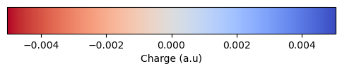
Text file
@jobs
task: scf
@end

@method settings
basis: def2-svp
xcfun: b3lyp
solvation model: cpcm
cpcm epsilon : 78.39
@end

@molecule
charge: 0
multiplicity: 1
xyz:
...
@end
SMD
The solvation model based on density (SMD) combines a self‑consistent reaction‑field description of the electrostatic polarization with empirically parametrized terms for cavitation, dispersion, and solvent–solute interactions based on the solute’s electron density, enabling accurate free‑energy predictions across a wide range of solvents. For further details, see Marenich et al. (2009).
In Veloxchem, the electrostatic contribution is determined using the CPCM model.
Python script
import veloxchem as vlx

molecule = vlx.Molecule.read_name("methanol")
basis = vlx.MolecularBasis.read(molecule, "def2-svp")

scf_drv = vlx.ScfRestrictedDriver()

scf_drv.solvation_model = "smd"
scf_drv.smd_solvent = "water"

scf_results = scf_drv.compute(molecule, basis)
Reading methanol from PubChem...
Reference: S. Kim, J. Chen, T. Cheng, A. Gindulyte, J. He, S. He, Q. Li, B. A. Shoemaker, P. A. Thiessen, B. Yu, L. Zaslavsky, J. Zhang, E. E. Bolton, Nucleic Acids Res., 2025, 53, D1516-D1525.
Please double-check the compound since names may refer to more than one record.
Self Consistent Field Driver Setup
====================================
Wave Function Model : Spin-Restricted Hartree-Fock
Initial Guess Model : Superposition of Atomic Densities
Convergence Accelerator : Two Level Direct Inversion of Iterative Subspace
Max. Number of Iterations : 50
Max. Number of Error Vectors : 10
Convergence Threshold : 1.0e-06
ERI Screening Threshold : 1.0e-12
Linear Dependence Threshold : 1.0e-06
Solvation Model : SMD
C-PCM Dielectric Constant : 78.355
C-PCM Points per Hydrogen Sphere: 110
C-PCM Points per non-H Sphere : 194
* Info * Using the SMD solvation model.
A. V. Marenich, C. J. Cramer, D. G. Truhlar, J. Phys. Chem. B, 2009, 113, 6378-6396.
* Info * Using C-PCM with the ISWIG discretization method.
A. W. Lange, J. M. Herbert, J. Chem. Phys. 2010, 133, 244111.
* Info * Starting Reduced Basis SCF calculation...
* Info * ...done. SCF energy in reduced basis set: -114.903255425992 a.u. Time: 0.91 sec.
Iter. | Hartree-Fock Energy | Energy Change | Gradient Norm | Max. Gradient | Density Change
--------------------------------------------------------------------------------------------
1 -114.961916642777 0.0000000000 0.11602781 0.01014808 0.00000000
2 -114.963369148940 -0.0014525062 0.02455942 0.00197338 0.03971934
3 -114.963433248364 -0.0000640994 0.00550944 0.00069305 0.00860649
4 -114.963438654537 -0.0000054062 0.00170200 0.00013333 0.00266958
5 -114.963439236346 -0.0000005818 0.00023663 0.00002385 0.00124713
6 -114.963439254814 -0.0000000185 0.00006531 0.00000599 0.00022792
7 -114.963439255630 -0.0000000008 0.00003712 0.00000349 0.00003723
8 -114.963439255793 -0.0000000002 0.00000470 0.00000048 0.00001329
9 -114.963439255847 -0.0000000001 0.00000087 0.00000009 0.00000319
*** SCF converged in 9 iterations. Time: 1.88 sec.
Spin-Restricted Hartree-Fock:
-----------------------------
Total Energy : -114.9634392558 a.u.
Electronic Energy : -155.2948915283 a.u.
SMD Solvation Energy : -0.0104447159 a.u
... ENP contribution : -0.0144129038 a.u.
... CDS contribution : 0.0039681879 a.u.
Nuclear Repulsion Energy : 40.3418969883 a.u.
------------------------------------
Gradient Norm : 0.0000008703 a.u.
Ground State Information
------------------------
Charge of Molecule : 0.0
Multiplicity (2S+1) : 1
Magnetic Quantum Number (M_S) : 0.0
Text file
@jobs
task: scf
@end

@method settings
basis: def2-svp
xcfun: b3lyp
solvation model: smd
smd solvent : water
@end

@molecule
charge: 0
multiplicity: 1
xyz:
...
@end
Explicit solvation
An explicit representation of the environment is available with the polarizable embedding (PE) model. Molecules in the environment are represented by site charges and polarizabilities. VeloxChem supports the PE model for:
SCF energies
linear response (UV/vis spectra and more)
The PE model is invoked in input files by giving the name of the associated potential file.
potfile_npe = """
@environment
units: angstrom
xyz:
O     -5.672000     2.390000    -4.911000  HOH_npe  1  OW
H     -6.099000     2.789000    -4.153000  HOH_npe  1  H1
H     -6.322000     2.449000    -5.611000  HOH_npe  1  H2
O      1.174000     1.993000    -1.482000  HOH_npe  2  OW
H      0.455000     2.074000    -0.855000  HOH_npe  2  H1
H      1.964000     2.142000    -0.963000  HOH_npe  2  H2
.
.
.
O     -7.851000    -3.106000     2.147000  HOH_npe  50  OW
H     -7.879000    -3.950000     1.697000  HOH_npe  50  H1
H     -8.589000    -2.616000     1.786000  HOH_npe  50  H2
@end

@charges
O   -0.83400000  HOH_npe
H    0.41700000  HOH_npe
H    0.41700000  HOH_npe
@end
"""

with open("solvent_npe.pot", "w") as f:
    f.write(potfile_npe)
potfile_pe = """
@environment
units: angstrom
xyz:
O -5.672000 2.390000 -4.911000 HOH_pe 1 OW
H -6.099000 2.789000 -4.153000 HOH_pe 1 H1
H -6.322000 2.449000 -5.611000 HOH_pe 1 H2
O 1.174000 1.993000 -1.482000 HOH_pe 2 OW
H 0.455000 2.074000 -0.855000 HOH_pe 2 H1
H 1.964000 2.142000 -0.963000 HOH_pe 2 H2
.
.
.
O -6.018000 6.513000 1.666000 HOH_npe 49 OW
H -6.698000 7.133000 1.402000 HOH_npe 49 H1
H -5.908000 6.663000 2.605000 HOH_npe 49 H2
@end
@charges
O -0.67444000 HOH_pe
H 0.33722000 HOH_pe
H 0.33722000 HOH_pe
O -0.83400000 HOH_npe
H 0.41700000 HOH_npe
H 0.41700000 HOH_npe
@end
@polarizabilities
O 5.73935000 0.00000000 0.00000000 5.73935000 0.00000000 5.73935000 HOH_pe
H 2.30839000 0.00000000 0.00000000 2.30839000 0.00000000 2.30839000 HOH_pe
H 2.30839000 0.00000000 0.00000000 2.30839000 0.00000000 2.30839000 HOH_pe
@end
"""
with open("solvent_pe.pot", "w") as f:
f.write(potfile_pe)
import py3Dmol

viewer = py3Dmol.view(width=600, height=400, linked=False)

h2o_xyz = """35
HS276
C        4.3399560215    0.0305428946    0.0828144786
C        4.4095576538    1.3683610158   -0.3235192595
H        3.5134027643    1.9937601903   -0.3924032993
N        5.5723395543    1.9197433737   -0.6488743924
C        6.6935279309    1.1757794133   -0.5864329168
H        7.6224068215    1.6875951052   -0.8616425839
C        6.7276910108   -0.1635918452   -0.2107845581
H        7.6695032300   -0.7162266137   -0.1924428573
C        5.5097537075   -0.7720747162    0.1336293537
C        5.1009824698   -2.0878240657    0.5406435604
H        5.7372998568   -2.9570654838    0.6892873628
C        3.7438801169   -2.0443763598    0.7226497610
H        3.0543062251   -2.8214265706    1.0462619034
N        3.2609508451   -0.7683360554    0.4549835483
C        1.9260075376   -0.3749845510    0.5283176588
S        0.6782993391   -1.3889716576   -0.1542613778
C        1.4061153730    0.7824770017    1.0601625728
H        2.0181143215    1.5416160613    1.5454703546
C       -0.0068851194    0.8477465652    0.9398680126
H       -0.6059313977    1.6741214421    1.3245241162
C       -0.5667478467   -0.2580211398    0.3294429618
C       -1.9604337493   -0.5533359638    0.0792123648
C       -2.5277285148   -1.7535587315   -0.3270277748
H       -1.9416881983   -2.6565543003   -0.5031604314
C       -3.9321104260   -1.6831753283   -0.4684223853
H       -4.5766877637   -2.5081858439   -0.7717042735
S       -3.1787442841    0.6764078755    0.2764099378
C       -4.4390511633   -0.4347565024   -0.1731766944
C       -5.8556810641   -0.0499048614   -0.2240721981
O       -6.7574530303   -0.7927799637   -0.5363405829
O       -6.0328437022    1.2420382988    0.1214233024
C       -7.3762795865    1.7182783197    0.1021539149
H       -8.0044633860    1.1450501374    0.8009438574
H       -7.3321515876    2.7714270760    0.4053723170
H       -7.8085678845    1.6284781442   -0.9060973811
"""

solvent_xyz = """150
water solvent
O     -5.672000     2.390000    -4.911000
H     -6.099000     2.789000    -4.153000
H     -6.322000     2.449000    -5.611000
O      1.174000     1.993000    -1.482000
H      0.455000     2.074000    -0.855000
H      1.964000     2.142000    -0.963000
O     -7.562000    -0.007000    -3.816000
H     -7.417000    -0.002000    -4.763000
H     -7.493000     0.912000    -3.558000
O      4.720000     2.913000    -3.470000
H      4.431000     2.735000    -4.365000
H      3.948000     2.745000    -2.930000
O      1.409000    -6.323000    -0.743000
H      0.743000    -6.705000    -0.172000
H      1.126000    -5.417000    -0.870000
O     -4.402000     1.138000    -2.230000
H     -5.203000     0.676000    -2.479000
H     -4.083000     0.668000    -1.460000
O      3.450000    -3.205000    -3.727000
H      3.640000    -4.043000    -3.304000
H      2.796000    -2.794000    -3.162000
O    -11.932000     1.045000     2.726000
H    -12.147000     1.345000     3.610000
H    -12.775000     0.801000     2.344000
O      6.421000    -2.296000     3.498000
H      6.522000    -1.527000     4.059000
H      7.037000    -2.936000     3.855000
O      6.492000    -5.683000     1.192000
H      6.315000    -4.742000     1.196000
H      6.210000    -5.983000     2.056000
O      3.182000    -0.144000     3.000000
H      3.680000    -0.571000     3.698000
H      2.275000    -0.163000     3.306000
O     10.335000     2.107000     2.815000
H     10.590000     2.278000     3.721000
H     10.070000     2.962000     2.475000
O      1.243000     4.026000     1.466000
H      1.933000     4.064000     0.804000
H      1.376000     3.186000     1.904000
O      7.353000     3.960000     1.428000
H      7.122000     4.445000     0.636000
H      6.921000     3.112000     1.324000
O     -0.167000    -3.859000     0.929000
H     -0.540000    -3.953000     1.806000
H      0.741000    -4.146000     1.022000
O     -2.563000    -1.777000     3.985000
H     -3.160000    -2.520000     3.894000
H     -1.695000    -2.174000     4.055000
O     -0.198000     0.919000    -3.501000
H     -0.421000     0.079000    -3.902000
H     -0.530000     0.853000    -2.606000
O     -0.812000    -2.339000    -2.398000
H     -0.905000    -3.080000    -2.996000
H     -0.364000    -1.668000    -2.913000
O     -4.686000    -4.040000    -2.308000
H     -3.760000    -3.848000    -2.160000
H     -5.150000    -3.292000    -1.933000
O     -8.539000     4.479000     2.210000
H     -8.404000     3.538000     2.095000
H     -8.831000     4.570000     3.117000
O      5.393000    -4.404000     4.731000
H      6.052000    -5.092000     4.633000
H      4.563000    -4.837000     4.532000
O      1.210000     2.523000     5.076000
H      0.643000     3.220000     4.746000
H      0.608000     1.891000     5.470000
O    -10.784000    -1.266000    -0.329000
H     -9.868000    -0.994000    -0.394000
H    -10.800000    -2.146000    -0.704000
O      8.747000    -0.111000     2.046000
H      9.209000     0.049000     1.224000
H      9.436000    -0.119000     2.711000
O     -5.495000    -3.818000     0.245000
H     -6.409000    -3.542000     0.178000
H     -5.240000    -4.024000    -0.655000
O      3.747000     4.848000    -0.533000
H      2.866000     4.753000    -0.894000
H      3.622000     4.823000     0.416000
O     -4.687000     0.733000     3.500000
H     -4.662000     0.206000     4.298000
H     -3.805000     0.660000     3.135000
O     -1.796000     0.340000     2.663000
H     -2.636000     0.782000     2.790000
H     -1.895000    -0.497000     3.118000
O      0.351000    -2.497000     5.213000
H      0.080000    -3.315000     4.795000
H     -0.410000    -1.923000     5.134000
O      4.193000     4.728000     3.519000
H      4.465000     5.575000     3.164000
H      4.987000     4.194000     3.501000
O      9.672000    -0.786000    -0.456000
H      9.202000    -1.077000    -1.238000
H     10.376000    -1.426000    -0.347000
O      6.075000     5.275000    -3.145000
H      5.188000     5.199000    -3.497000
H      6.273000     6.210000    -3.196000
O      7.916000     2.509000    -4.256000
H      8.024000     1.974000    -5.043000
H      8.635000     2.242000    -3.684000
O      8.531000     4.047000    -2.078000
H      9.121000     4.282000    -2.794000
H      8.149000     3.212000    -2.345000
O      5.804000    -0.819000    -5.002000
H      6.693000    -0.763000    -5.353000
H      5.655000     0.031000    -4.588000
O      5.627000     1.092000     2.883000
H      5.959000     0.251000     2.569000
H      5.073000     0.868000     3.630000
O      3.899000    -0.985000    -2.382000
H      3.319000    -1.142000    -3.127000
H      4.198000    -1.857000    -2.122000
O      9.979000     4.138000     0.834000
H     10.413000     3.442000     1.328000
H      9.745000     4.790000     1.494000
O     -9.211000    -0.316000     1.813000
H     -9.462000    -0.901000     2.528000
H     -8.541000     0.253000     2.193000
O     -7.317000     0.233000     3.510000
H     -7.721000    -0.414000     2.933000
H     -6.848000     0.822000     2.920000
O      5.410000     0.333000     5.529000
H      5.548000    -0.006000     6.413000
H      4.778000    -0.269000     5.136000
O      9.233000    -4.492000     2.022000
H      8.767000    -4.312000     2.839000
H      9.317000    -5.445000     1.998000
O     -3.699000     3.318000     0.684000
H     -2.960000     3.399000     1.287000
H     -4.306000     4.007000     0.956000
O     -4.961000    -4.974000     2.628000
H     -5.362000    -5.229000     1.797000
H     -4.134000    -5.457000     2.653000
O     -2.552000    -0.428000    -3.959000
H     -2.788000     0.448000    -4.264000
H     -3.390000    -0.854000    -3.779000
O     -8.214000    -3.642000    -1.366000
H     -8.474000    -3.129000    -0.601000
H     -8.954000    -4.228000    -1.524000
O     -5.399000     4.648000    -2.415000
H     -5.405000     3.717000    -2.192000
H     -5.118000     5.084000    -1.610000
O     -1.605000     0.714000     6.024000
H     -1.508000     1.009000     6.930000
H     -1.010000    -0.032000     5.950000
O     -6.018000     6.513000     1.666000
H     -6.698000     7.133000     1.402000
H     -5.908000     6.663000     2.605000
O     -7.851000    -3.106000     2.147000
H     -7.879000    -3.950000     1.697000
H     -8.589000    -2.616000     1.786000
"""

# Load as XYZ so the parser knows the format explicitly
viewer.addModel(h2o_xyz, 'xyz')       # model 0: solute
viewer.addModel(solvent_xyz, 'xyz')   # model 1: solvent

# Clear any default styling, then style per model
viewer.setStyle({}, {})  # reset

viewer.addStyle({'model': 0}, {'stick': {'radius': 0.30, 'colorscheme': 'Jmol'}})
viewer.addStyle({'model': 1}, {'stick': {'radius': 0.10, 'color': '#9bbcff'}})

# Outline and view settings
viewer.setViewStyle({"style": "outline", "color": "black", "width": 0.1})

# Rotate and focus on solute
viewer.rotate(45, "x")
viewer.zoomTo({'model': 0})

viewer.show()Python script
import veloxchem as vlx

solute_xyz = """35
HS276
C        4.3399560215    0.0305428946    0.0828144786
C        4.4095576538    1.3683610158   -0.3235192595
H        3.5134027643    1.9937601903   -0.3924032993
N        5.5723395543    1.9197433737   -0.6488743924
C        6.6935279309    1.1757794133   -0.5864329168
H        7.6224068215    1.6875951052   -0.8616425839
C        6.7276910108   -0.1635918452   -0.2107845581
H        7.6695032300   -0.7162266137   -0.1924428573
C        5.5097537075   -0.7720747162    0.1336293537
C        5.1009824698   -2.0878240657    0.5406435604
H        5.7372998568   -2.9570654838    0.6892873628
C        3.7438801169   -2.0443763598    0.7226497610
H        3.0543062251   -2.8214265706    1.0462619034
N        3.2609508451   -0.7683360554    0.4549835483
C        1.9260075376   -0.3749845510    0.5283176588
S        0.6782993391   -1.3889716576   -0.1542613778
C        1.4061153730    0.7824770017    1.0601625728
H        2.0181143215    1.5416160613    1.5454703546
C       -0.0068851194    0.8477465652    0.9398680126
H       -0.6059313977    1.6741214421    1.3245241162
C       -0.5667478467   -0.2580211398    0.3294429618
C       -1.9604337493   -0.5533359638    0.0792123648
C       -2.5277285148   -1.7535587315   -0.3270277748
H       -1.9416881983   -2.6565543003   -0.5031604314
C       -3.9321104260   -1.6831753283   -0.4684223853
H       -4.5766877637   -2.5081858439   -0.7717042735
S       -3.1787442841    0.6764078755    0.2764099378
C       -4.4390511633   -0.4347565024   -0.1731766944
C       -5.8556810641   -0.0499048614   -0.2240721981
O       -6.7574530303   -0.7927799637   -0.5363405829
O       -6.0328437022    1.2420382988    0.1214233024
C       -7.3762795865    1.7182783197    0.1021539149
H       -8.0044633860    1.1450501374    0.8009438574
H       -7.3321515876    2.7714270760    0.4053723170
H       -7.8085678845    1.6284781442   -0.9060973811
"""

molecule = vlx.Molecule.read_xyz_string(solute_xyz)
basis = vlx.MolecularBasis.read(molecule, "def2-svp")

scf_drv = vlx.ScfRestrictedDriver()

scf_drv.potfile = "solvent.pot"

scf_results = scf_drv.compute(molecule, basis)
Text file
@jobs
task: scf
@end

@method settings
basis: aug-cc-pvdz
potfile: solvent.pot
@end

@molecule
charge: 0
multiplicity: 1
xyz:
C        4.3399560215    0.0305428946    0.0828144786
C        4.4095576538    1.3683610158   -0.3235192595
H        3.5134027643    1.9937601903   -0.3924032993
N        5.5723395543    1.9197433737   -0.6488743924
C        6.6935279309    1.1757794133   -0.5864329168
H        7.6224068215    1.6875951052   -0.8616425839
C        6.7276910108   -0.1635918452   -0.2107845581
H        7.6695032300   -0.7162266137   -0.1924428573
C        5.5097537075   -0.7720747162    0.1336293537
C        5.1009824698   -2.0878240657    0.5406435604
H        5.7372998568   -2.9570654838    0.6892873628
C        3.7438801169   -2.0443763598    0.7226497610
H        3.0543062251   -2.8214265706    1.0462619034
N        3.2609508451   -0.7683360554    0.4549835483
C        1.9260075376   -0.3749845510    0.5283176588
S        0.6782993391   -1.3889716576   -0.1542613778
C        1.4061153730    0.7824770017    1.0601625728
H        2.0181143215    1.5416160613    1.5454703546
C       -0.0068851194    0.8477465652    0.9398680126
H       -0.6059313977    1.6741214421    1.3245241162
C       -0.5667478467   -0.2580211398    0.3294429618
C       -1.9604337493   -0.5533359638    0.0792123648
C       -2.5277285148   -1.7535587315   -0.3270277748
H       -1.9416881983   -2.6565543003   -0.5031604314
C       -3.9321104260   -1.6831753283   -0.4684223853
H       -4.5766877637   -2.5081858439   -0.7717042735
S       -3.1787442841    0.6764078755    0.2764099378
C       -4.4390511633   -0.4347565024   -0.1731766944
C       -5.8556810641   -0.0499048614   -0.2240721981
O       -6.7574530303   -0.7927799637   -0.5363405829
O       -6.0328437022    1.2420382988    0.1214233024
C       -7.3762795865    1.7182783197    0.1021539149
H       -8.0044633860    1.1450501374    0.8009438574
H       -7.3321515876    2.7714270760    0.4053723170
H       -7.8085678845    1.6284781442   -0.9060973811
@end
Non-polarizable embedding
Potential file
The potential file named solvent_npe.pot in this example takes the following form, where all water molecules are treated as non-polarizable.
print(potfile_npe)
@environment
units: angstrom
xyz:
O     -5.672000     2.390000    -4.911000  HOH_npe  1  OW
H     -6.099000     2.789000    -4.153000  HOH_npe  1  H1
H     -6.322000     2.449000    -5.611000  HOH_npe  1  H2
O      1.174000     1.993000    -1.482000  HOH_npe  2  OW
H      0.455000     2.074000    -0.855000  HOH_npe  2  H1
H      1.964000     2.142000    -0.963000  HOH_npe  2  H2
.
.
.
O     -7.851000    -3.106000     2.147000  HOH_npe  50  OW
H     -7.879000    -3.950000     1.697000  HOH_npe  50  H1
H     -8.589000    -2.616000     1.786000  HOH_npe  50  H2
@end

@charges
O   -0.83400000  HOH_npe
H    0.41700000  HOH_npe
H    0.41700000  HOH_npe
@end
Polarizable embedding
The following potential file solvent_pe.pot contains most water molecules treated as polarizable and others as non-polarizable.
print(potfile_pe)
@environment
units: angstrom
xyz:
O     -5.672000     2.390000    -4.911000  HOH_pe  1  OW
H     -6.099000     2.789000    -4.153000  HOH_pe  1  H1
H     -6.322000     2.449000    -5.611000  HOH_pe  1  H2
O      1.174000     1.993000    -1.482000  HOH_pe  2  OW
H      0.455000     2.074000    -0.855000  HOH_pe  2  H1
H      1.964000     2.142000    -0.963000  HOH_pe  2  H2
.
.
.
O     -6.018000     6.513000     1.666000  HOH_npe  49  OW
H     -6.698000     7.133000     1.402000  HOH_npe  49  H1
H     -5.908000     6.663000     2.605000  HOH_npe  49  H2
@end

@charges
O   -0.67444000  HOH_pe
H    0.33722000  HOH_pe
H    0.33722000  HOH_pe
O   -0.83400000  HOH_npe
H    0.41700000  HOH_npe
H    0.41700000  HOH_npe
@end

@polarizabilities
O    5.73935000   0.00000000   0.00000000   5.73935000   0.00000000   5.73935000  HOH_pe
H    2.30839000   0.00000000   0.00000000   2.30839000   0.00000000   2.30839000  HOH_pe
H    2.30839000   0.00000000   0.00000000   2.30839000   0.00000000   2.30839000  HOH_pe
@end
The polarizability components are listed in the order xx, xy, xz, yy, yz, zz.
- Tomasi, J., Mennucci, B., & Cammi, R. (2005). Quantum Mechanical Continuum Solvation Models. Chem. Rev., 105(8), 2999–3094. 10.1021/cr9904009
- Marenich, A. V., Cramer, C. J., & Truhlar, D. G. (2009). Universal Solvation Model Based on Solute Electron Density and on a Continuum Model of the Solvent Defined by the Bulk Dielectric Constant and Atomic Surface Tensions. J. Phys. Chem. B, 113(18), 6378–6396. 10.1021/jp810292n