From a notebook cell
import veloxchem as vlx

molecule = vlx.Molecule.read_smiles('CCO')
basis = vlx.MolecularBasis.read(molecule, 'def2-svp')

scf_drv = vlx.ScfRestrictedDriver()
scf_drv.xcfun = 'b3lyp'
scf_results = scf_drv.compute(molecule, basis)

rsp_drv = vlx.lreigensolver.LinearResponseEigenSolver()
rsp_drv.nstates = 10
rsp_results = rsp_drv.compute(molecule, basis, scf_results)
                                            Self Consistent Field Driver Setup
                                           ====================================

                   Wave Function Model             : Spin-Restricted Kohn-Sham
                   Initial Guess Model             : Superposition of Atomic Densities
                   Convergence Accelerator         : Two Level Direct Inversion of Iterative Subspace
                   Max. Number of Iterations       : 50
                   Max. Number of Error Vectors    : 10
                   Convergence Threshold           : 1.0e-06
                   ERI Screening Threshold         : 1.0e-12
                   Linear Dependence Threshold     : 1.0e-06
                   Exchange-Correlation Functional : B3LYP
                   Molecular Grid Level            : 4

* Info * Using the B3LYP functional.

         P. J. Stephens, F. J. Devlin, C. F. Chabalowski, and M. J. Frisch.,  J. Phys. Chem. 98, 11623 (1994)

* Info * Using the Libxc library (v7.0.0).

         S. Lehtola, C. Steigemann, M. J.T. Oliveira, and M. A.L. Marques.,  SoftwareX 7, 1–5 (2018)

* Info * Using the following algorithm for XC numerical integration.

         J. Kussmann, H. Laqua and C. Ochsenfeld, J. Chem. Theory Comput. 2021, 17, 1512-1521

* Info * Starting Reduced Basis SCF calculation...
* Info * ...done. SCF energy in reduced basis set: -153.878486392936 a.u. Time: 0.20 sec.


               Iter. |    Kohn-Sham Energy | Energy Change | Gradient Norm | Max. Gradient | Density Change
               --------------------------------------------------------------------------------------------
                  1      -154.914064502408    0.0000000000      0.25700154      0.02179011      0.00000000
                  2      -154.917228200392   -0.0031636980      0.18477397      0.01179506      0.14535754
                  3      -154.921419464512   -0.0041912641      0.03153015      0.00159927      0.06527732
                  4      -154.921522198651   -0.0001027341      0.00963180      0.00077432      0.01040150
                  5      -154.921530557133   -0.0000083585      0.00173197      0.00010436      0.00336227
                  6      -154.921530851578   -0.0000002944      0.00029569      0.00002451      0.00063152
                  7      -154.921530862992   -0.0000000114      0.00003877      0.00000229      0.00013434
                  8      -154.921530863151   -0.0000000002      0.00001670      0.00000085      0.00001563
                  9      -154.921530863185   -0.0000000000      0.00000165      0.00000009      0.00000567
                 10      -154.921530863186   -0.0000000000      0.00000015      0.00000001      0.00000083

               *** SCF converged in 10 iterations. Time: 2.08 sec.

               Spin-Restricted Kohn-Sham:
               --------------------------
               Total Energy                       :     -154.9215308632 a.u.
               Electronic Energy                  :     -236.6490992715 a.u.
               Nuclear Repulsion Energy           :       81.7275684083 a.u.
               ------------------------------------
               Gradient Norm                      :        0.0000001479 a.u.


               Ground State Information
               ------------------------
               Charge of Molecule            :  0.0
               Multiplicity (2S+1)           :  1
               Magnetic Quantum Number (M_S) :  0.0


                                            Linear Response EigenSolver Setup
                                           ===================================

                               Number of States                : 10
                               Max. Number of Iterations       : 150
                               Convergence Threshold           : 1.0e-04
                               ERI Screening Threshold         : 1.0e-12
                               Exchange-Correlation Functional : B3LYP
                               Molecular Grid Level            : 4

* Info * Using the B3LYP functional.

         P. J. Stephens, F. J. Devlin, C. F. Chabalowski, and M. J. Frisch.,  J. Phys. Chem. 98, 11623 (1994)

* Info * Using the Libxc library (v7.0.0).

         S. Lehtola, C. Steigemann, M. J.T. Oliveira, and M. A.L. Marques.,  SoftwareX 7, 1–5 (2018)

* Info * Using the following algorithm for XC numerical integration.

         J. Kussmann, H. Laqua and C. Ochsenfeld, J. Chem. Theory Comput. 2021, 17, 1512-1521

* Info * 30 gerade trial vectors in reduced space
* Info * 30 ungerade trial vectors in reduced space

               *** Iteration:   1 * Residuals (Max,Min): 1.85e-01 and 6.38e-02

* Info * 40 gerade trial vectors in reduced space
* Info * 40 ungerade trial vectors in reduced space

               *** Iteration:   2 * Residuals (Max,Min): 3.03e-02 and 1.21e-02

* Info * 50 gerade trial vectors in reduced space
* Info * 50 ungerade trial vectors in reduced space

               *** Iteration:   3 * Residuals (Max,Min): 4.74e-03 and 1.81e-03

* Info * 60 gerade trial vectors in reduced space
* Info * 60 ungerade trial vectors in reduced space

               *** Iteration:   4 * Residuals (Max,Min): 5.42e-04 and 2.22e-04

* Info * 70 gerade trial vectors in reduced space
* Info * 70 ungerade trial vectors in reduced space

               *** Iteration:   5 * Residuals (Max,Min): 5.22e-05 and 1.71e-05

               *** Linear response converged in 5 iterations. Time: 12.18 sec


               Electric Transition Dipole Moments (dipole length, a.u.)
               --------------------------------------------------------
                                                X            Y            Z
               Excited State    S1:      0.170366    -0.067360     0.043499
               Excited State    S2:     -0.112757     0.191976    -0.278437
               Excited State    S3:      0.120200    -0.053494    -0.157485
               Excited State    S4:     -0.112307     0.318122     0.274489
               Excited State    S5:      0.242704     0.323168     0.199478
               Excited State    S6:      0.008061     0.148086    -0.217363
               Excited State    S7:      0.264323    -0.173816     0.003618
               Excited State    S8:     -0.029582     0.217407    -0.482774
               Excited State    S9:      0.043381    -0.082979     0.034737
               Excited State   S10:      0.366135    -0.165059     0.106723

               Electric Transition Dipole Moments (dipole velocity, a.u.)
               ----------------------------------------------------------
                                                X            Y            Z
               Excited State    S1:      0.224330    -0.249331    -0.055966
               Excited State    S2:     -0.060052     0.082726    -0.312042
               Excited State    S3:      0.221088    -0.029449    -0.159829
               Excited State    S4:     -0.074165     0.280613     0.295005
               Excited State    S5:      0.237315     0.376183     0.257681
               Excited State    S6:      0.080653     0.187060    -0.191254
               Excited State    S7:      0.282642    -0.149118    -0.028326
               Excited State    S8:     -0.029870     0.213960    -0.508216
               Excited State    S9:      0.041042    -0.084370     0.046230
               Excited State   S10:      0.368957    -0.168999     0.113123

               Magnetic Transition Dipole Moments (a.u.)
               -----------------------------------------
                                                X            Y            Z
               Excited State    S1:      0.386044     0.119530    -0.040394
               Excited State    S2:     -0.039851     0.064214    -0.021148
               Excited State    S3:     -0.162978     0.533976     0.025879
               Excited State    S4:      0.029758     0.002127    -0.032410
               Excited State    S5:     -0.229965     0.016255    -0.093218
               Excited State    S6:      0.000430     0.020861     0.451976
               Excited State    S7:      0.116200     0.188254     0.238687
               Excited State    S8:     -0.401307    -0.133265    -0.130288
               Excited State    S9:      0.038538    -0.024849    -0.155939
               Excited State   S10:      0.162664     0.148427    -0.263220

               One-Photon Absorption
               ---------------------
               Excited State    S1:      0.25657814 a.u.      6.98185 eV    Osc.Str.    0.0061
               Excited State    S2:      0.30999769 a.u.      8.43547 eV    Osc.Str.    0.0263
               Excited State    S3:      0.31640957 a.u.      8.60994 eV    Osc.Str.    0.0089
               Excited State    S4:      0.33276709 a.u.      9.05505 eV    Osc.Str.    0.0420
               Excited State    S5:      0.34369112 a.u.      9.35231 eV    Osc.Str.    0.0465
               Excited State    S6:      0.36134944 a.u.      9.83282 eV    Osc.Str.    0.0167
               Excited State    S7:      0.36299244 a.u.      9.87753 eV    Osc.Str.    0.0242
               Excited State    S8:      0.37099871 a.u.     10.09539 eV    Osc.Str.    0.0696
               Excited State    S9:      0.37686861 a.u.     10.25512 eV    Osc.Str.    0.0025
               Excited State   S10:      0.38367771 a.u.     10.44040 eV    Osc.Str.    0.0442

               Electronic Circular Dichroism
               -----------------------------
               Excited State    S1:     Rot.Str.      0.059060 a.u.    27.8433 [10**(-40) cgs]
               Excited State    S2:     Rot.Str.      0.014304 a.u.     6.7437 [10**(-40) cgs]
               Excited State    S3:     Rot.Str.     -0.055894 a.u.   -26.3509 [10**(-40) cgs]
               Excited State    S4:     Rot.Str.     -0.011171 a.u.    -5.2666 [10**(-40) cgs]
               Excited State    S5:     Rot.Str.     -0.072480 a.u.   -34.1702 [10**(-40) cgs]
               Excited State    S6:     Rot.Str.     -0.082505 a.u.   -38.8965 [10**(-40) cgs]
               Excited State    S7:     Rot.Str.     -0.001990 a.u.    -0.9383 [10**(-40) cgs]
               Excited State    S8:     Rot.Str.      0.049688 a.u.    23.4251 [10**(-40) cgs]
               Excited State    S9:     Rot.Str.     -0.003531 a.u.    -1.6647 [10**(-40) cgs]
               Excited State   S10:     Rot.Str.      0.005156 a.u.     2.4306 [10**(-40) cgs]

               Character of excitations:

               Excited state 1
               ---------------
               HOMO     -> LUMO        -0.9824

               Excited state 2
               ---------------
               HOMO     -> LUMO+1      -0.9670

               Excited state 3
               ---------------
               HOMO-1   -> LUMO         0.9828

               Excited state 4
               ---------------
               HOMO     -> LUMO+2       0.9881

               Excited state 5
               ---------------
               HOMO     -> LUMO+3      -0.9808

               Excited state 6
               ---------------
               HOMO-1   -> LUMO+1       0.7326
               HOMO     -> LUMO+4      -0.5321
               HOMO-2   -> LUMO        -0.3830

               Excited state 7
               ---------------
               HOMO     -> LUMO+4       0.8200
               HOMO-1   -> LUMO+1       0.5162

               Excited state 8
               ---------------
               HOMO-2   -> LUMO         0.8857
               HOMO-1   -> LUMO+1       0.4213

               Excited state 9
               ---------------
               HOMO     -> LUMO+5       0.9887

               Excited state 10
               ----------------
               HOMO-3   -> LUMO         0.8995
               HOMO-1   -> LUMO+2       0.3820
rsp_drv.plot(rsp_results)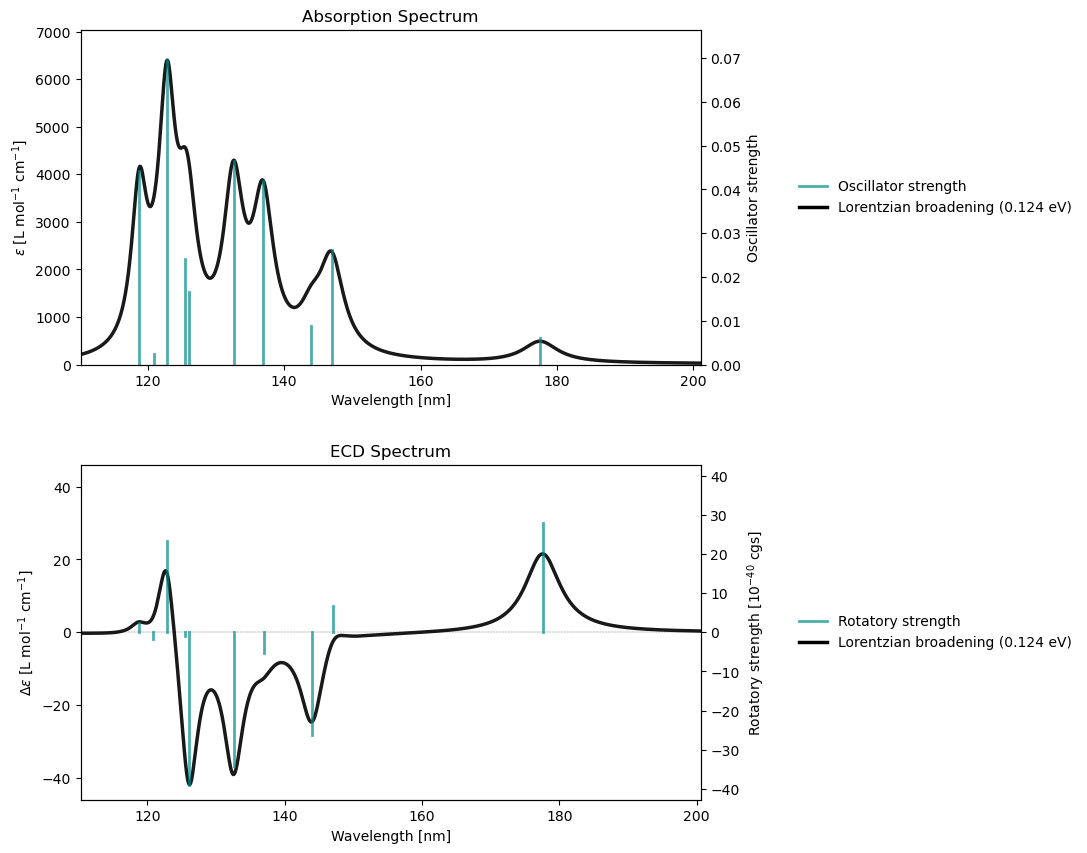
From an h5 file
rsp_results = vlx.read_results("../output_files/alanine-ecd.h5", label="rsp")
rsp_drv.plot_ecd(rsp_results)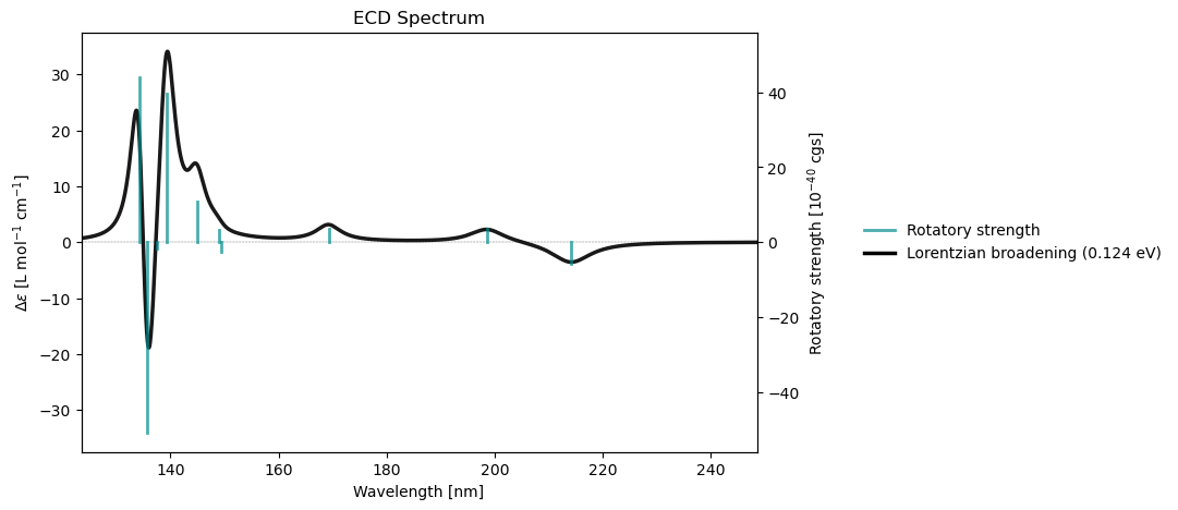
VIbrational Spectrum
From a notebook cell
molecule = vlx.Molecule.read_smiles('CCO')
basis = vlx.MolecularBasis.read(molecule, 'def2-svp')

scf_drv = vlx.ScfRestrictedDriver()
scf_drv.xcfun = 'b3lyp'
scf_results = scf_drv.compute(molecule, basis)

vib_drv = vlx.VibrationalAnalysis(scf_drv)
vib_results = vib_drv.compute(molecule, basis)
Self Consistent Field Driver Setup
====================================
Wave Function Model : Spin-Restricted Kohn-Sham
Initial Guess Model : Superposition of Atomic Densities
Convergence Accelerator : Two Level Direct Inversion of Iterative Subspace
Max. Number of Iterations : 50
Max. Number of Error Vectors : 10
Convergence Threshold : 1.0e-06
ERI Screening Threshold : 1.0e-12
Linear Dependence Threshold : 1.0e-06
Exchange-Correlation Functional : B3LYP
Molecular Grid Level : 4
* Info * Using the B3LYP functional.
P. J. Stephens, F. J. Devlin, C. F. Chabalowski, and M. J. Frisch., J. Phys. Chem. 98, 11623 (1994)
* Info * Using the Libxc library (v7.0.0).
S. Lehtola, C. Steigemann, M. J.T. Oliveira, and M. A.L. Marques., SoftwareX 7, 1–5 (2018)
* Info * Using the following algorithm for XC numerical integration.
J. Kussmann, H. Laqua and C. Ochsenfeld, J. Chem. Theory Comput. 2021, 17, 1512-1521
* Info * Starting Reduced Basis SCF calculation...
* Info * ...done. SCF energy in reduced basis set: -153.878486356222 a.u. Time: 0.16 sec.
Iter. | Kohn-Sham Energy | Energy Change | Gradient Norm | Max. Gradient | Density Change
--------------------------------------------------------------------------------------------
1 -154.914062365295 0.0000000000 0.25699951 0.02179046 0.00000000
2 -154.917225981603 -0.0031636163 0.18477285 0.01179468 0.14535564
3 -154.921417167139 -0.0041911855 0.03153154 0.00159950 0.06527629
4 -154.921519907108 -0.0001027400 0.00963290 0.00077441 0.01040181
5 -154.921528267551 -0.0000083604 0.00173186 0.00010435 0.00336258
6 -154.921528561971 -0.0000002944 0.00029568 0.00002451 0.00063151
7 -154.921528573385 -0.0000000114 0.00003877 0.00000229 0.00013434
8 -154.921528573543 -0.0000000002 0.00001670 0.00000085 0.00001563
9 -154.921528573578 -0.0000000000 0.00000165 0.00000009 0.00000567
10 -154.921528573578 -0.0000000000 0.00000015 0.00000001 0.00000083
*** SCF converged in 10 iterations. Time: 1.83 sec.
Spin-Restricted Kohn-Sham:
--------------------------
Total Energy : -154.9215285736 a.u.
Electronic Energy : -236.6491077379 a.u.
Nuclear Repulsion Energy : 81.7275791644 a.u.
------------------------------------
Gradient Norm : 0.0000001479 a.u.
Ground State Information
------------------------
Charge of Molecule : 0.0
Multiplicity (2S+1) : 1
Magnetic Quantum Number (M_S) : 0.0
Vibrational Analysis Driver
=============================
The following will be computed:
- Vibrational frequencies and normal modes
- Force constants
- IR intensities
SCF Hessian Driver Setup
==========================
Hessian Type : Analytical
* Info * Computing analytical Hessian...
Reference: P. Deglmann, F. Furche, R. Ahlrichs, Chem. Phys. Lett. 2002, 362, 511-518.
* Info * Using the B3LYP functional.
P. J. Stephens, F. J. Devlin, C. F. Chabalowski, and M. J. Frisch., J. Phys. Chem. 98, 11623 (1994)
* Info * Using the Libxc library (v7.0.0).
S. Lehtola, C. Steigemann, M. J.T. Oliveira, and M. A.L. Marques., SoftwareX 7, 1–5 (2018)
* Info * Using the following algorithm for XC numerical integration.
J. Kussmann, H. Laqua and C. Ochsenfeld, J. Chem. Theory Comput. 2021, 17, 1512-1521
* Info * CPHF/CPKS integral derivatives computed in 5.47 sec.
* Info * CPHF/CPKS right-hand side computed in 5.28 sec.
Coupled-Perturbed Kohn-Sham Solver Setup
------------------------------------------
Solver Type : Iterative Subspace Algorithm
Max. Number of Iterations : 150
Convergence Threshold : 1.0e-04
Exchange-Correlation Functional : B3LYP
Molecular Grid Level : 4
* Info * 24 trial vectors in reduced space
*** Iteration: 1 * Residuals (Max,Min): 3.72e-01 and 1.30e-01
* Info * 48 trial vectors in reduced space
*** Iteration: 2 * Residuals (Max,Min): 3.26e-02 and 1.09e-02
* Info * 72 trial vectors in reduced space
*** Iteration: 3 * Residuals (Max,Min): 2.15e-03 and 6.02e-04
* Info * 89 trial vectors in reduced space
*** Iteration: 4 * Residuals (Max,Min): 1.44e-04 and 4.22e-05
* Info * 107 trial vectors in reduced space
*** Iteration: 5 * Residuals (Max,Min): 9.42e-05 and 4.34e-06
*** Coupled-Perturbed Kohn-Sham converged in 5 iterations. Time: 28.90 sec
* Info * First order derivative contributions to the Hessian computed in 0.00 sec.
* Info * Second order derivative contributions to the Hessian computed in 22.79 sec.
*** Time spent in Hessian calculation: 51.74 sec ***
Free Energy Analysis
======================
Note: Rotational symmetry is set to 1 regardless of true symmetry
No Imaginary Frequencies
Free energy contributions calculated at @ 298.15 K:
Zero-point vibrational energy: 50.1144 kcal/mol
H (Trans + Rot + Vib = Tot): 1.4812 + 0.8887 + 0.6064 = 2.9763 kcal/mol
S (Trans + Rot + Vib = Tot): 37.4322 + 22.3320 + 2.8170 = 62.5812 cal/mol/K
TS (Trans + Rot + Vib = Tot): 11.1604 + 6.6583 + 0.8399 = 18.6586 kcal/mol
Ground State Electronic Energy : E0 = -154.92152857 au ( -97214.7269 kcal/mol)
Free Energy Correction (Harmonic) : ZPVE + [H-TS]_T,R,V = 0.05487117 au ( 34.4322 kcal/mol)
Gibbs Free Energy (Harmonic) : E0 + ZPVE + [H-TS]_T,R,V = -154.86665741 au ( -97180.2947 kcal/mol)
Vibrational Analysis
======================
* Info * The 5 dominant normal modes are printed below.
Vibrational Mode 3
----------------------------------------------------
Harmonic frequency: 645.87 cm**-1
Reduced mass: 1.1162 amu
Force constant: 0.2743 mdyne/A
IR intensity: 123.0915 km/mol
Normal mode:
X Y Z
1 C 0.0207 0.0129 -0.0043
2 C -0.0152 -0.0224 -0.0152
3 O -0.0436 0.0559 0.0324
4 H -0.0095 0.0370 0.0099
5 H 0.1078 -0.0066 -0.0175
6 H 0.0413 0.0581 0.0668
7 H -0.0341 -0.0585 0.0647
8 H -0.0247 -0.0656 -0.0812
9 H 0.5469 -0.7381 -0.3243
Vibrational Mode 7
----------------------------------------------------
Harmonic frequency: 1132.52 cm**-1
Reduced mass: 1.6310 amu
Force constant: 1.2325 mdyne/A
IR intensity: 82.0998 km/mol
Normal mode:
X Y Z
1 C 0.0436 0.0744 -0.0306
2 C -0.0469 -0.1091 0.1128
3 O -0.0245 0.0404 -0.1163
4 H -0.2179 -0.0086 0.0222
5 H -0.2290 0.0615 0.1263
6 H 0.2367 -0.2700 0.0090
7 H 0.1529 0.0482 -0.2498
8 H 0.1839 -0.0207 0.5890
9 H 0.3010 -0.0382 0.3721
Vibrational Mode 12
----------------------------------------------------
Harmonic frequency: 1443.60 cm**-1
Reduced mass: 1.1421 amu
Force constant: 1.4024 mdyne/A
IR intensity: 46.2920 km/mol
Normal mode:
X Y Z
1 C 0.0229 0.0119 -0.0026
2 C -0.0599 -0.0287 0.0057
3 O 0.0589 0.0339 0.0242
4 H -0.2544 -0.2669 -0.0041
5 H 0.0668 -0.1295 0.1873
6 H -0.1339 0.1130 -0.1644
7 H -0.0768 0.0697 -0.1510
8 H 0.2030 -0.1588 0.3600
9 H -0.2985 0.0350 -0.6479
Vibrational Mode 16
----------------------------------------------------
Harmonic frequency: 2931.05 cm**-1
Reduced mass: 1.0652 amu
Force constant: 5.3916 mdyne/A
IR intensity: 72.4279 km/mol
Normal mode:
X Y Z
1 C -0.0058 -0.0008 -0.0061
2 C -0.0033 0.0516 0.0497
3 O 0.0004 -0.0006 0.0020
4 H 0.0195 -0.0239 0.0981
5 H 0.0028 0.0060 0.0022
6 H 0.0525 0.0286 -0.0322
7 H -0.2439 -0.7619 -0.4686
8 H 0.2681 0.1592 -0.1504
9 H 0.0030 -0.0028 0.0003
Vibrational Mode 19
----------------------------------------------------
Harmonic frequency: 3037.43 cm**-1
Reduced mass: 1.1032 amu
Force constant: 5.9967 mdyne/A
IR intensity: 42.2175 km/mol
Normal mode:
X Y Z
1 C 0.0146 0.0223 -0.0869
2 C 0.0153 0.0099 -0.0089
3 O -0.0007 -0.0004 0.0007
4 H 0.2008 -0.2034 0.7252
5 H 0.0576 0.1716 0.0905
6 H -0.4346 -0.2312 0.2301
7 H -0.0065 -0.0230 -0.0124
8 H -0.1705 -0.0913 0.0966
9 H 0.0083 0.0012 0.0006
vib_drv.plot(vib_results)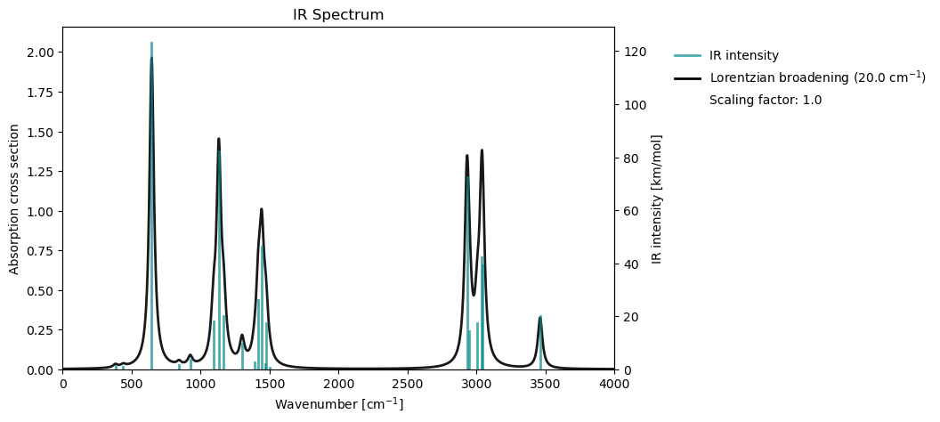
From an h5 file
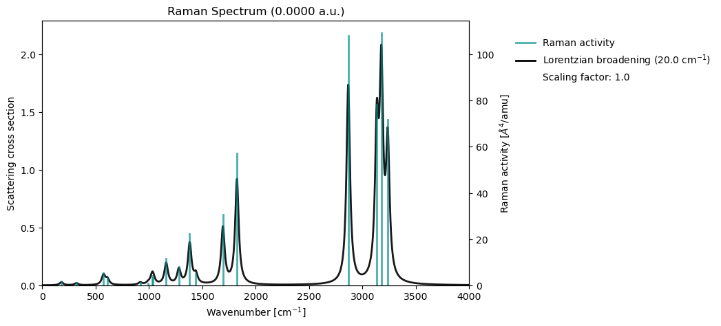
vib_results = vlx.read_results("../output_files/acro-raman.h5", label="vib")
vib_drv.plot_raman(vib_results)