Ensembles - VeloxChem Docs

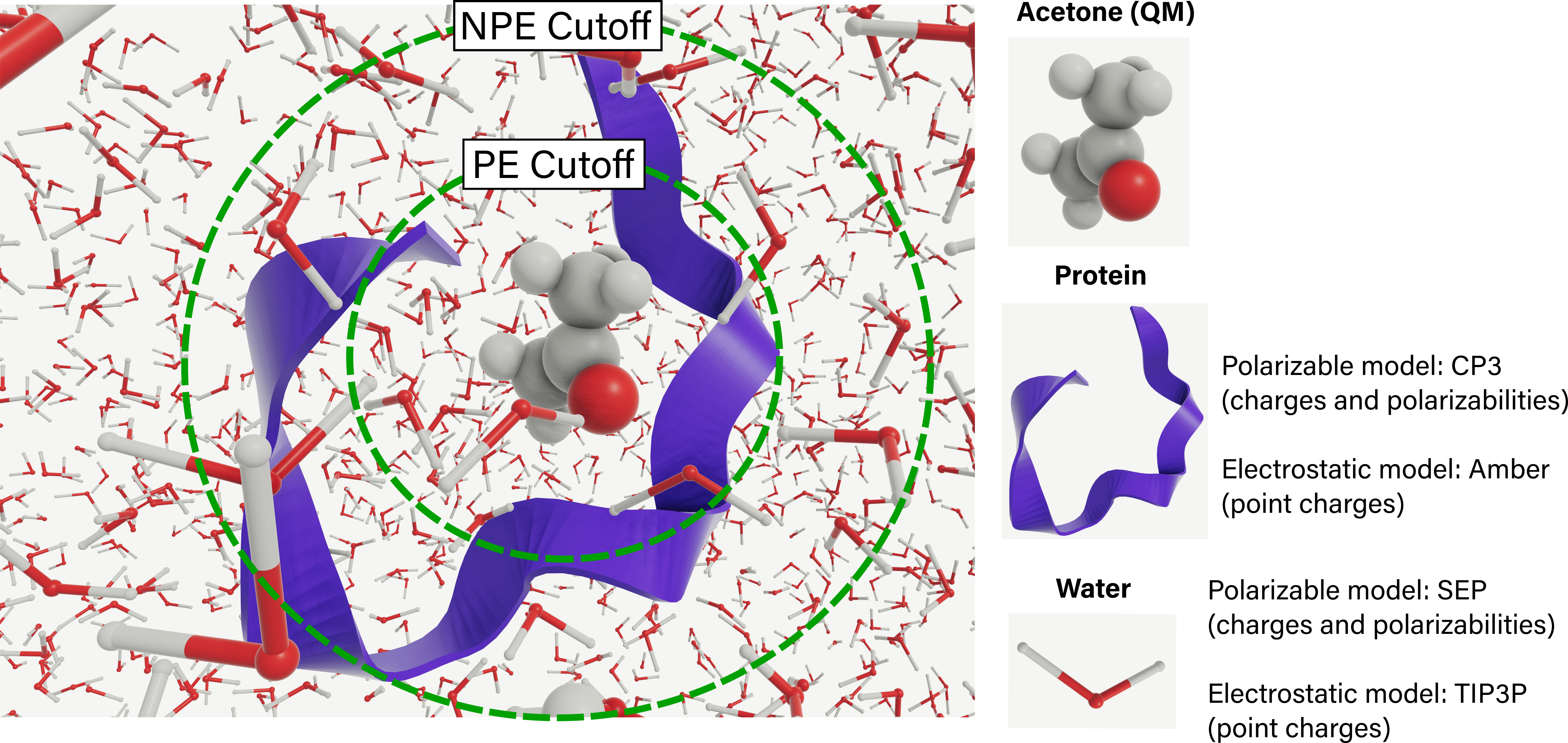
Complex environments containing proteins, water, and ions like the one shown below can be represented explicitly using:

Polarizable embedding (PE), where molecules in the environment are represented by site charges and polarizabilities.
Non-polarizable embedding (NPE), where the environment is represented by point charges only.

import py3Dmol

with open("../input_files/alpha-helix-acetone-water.pdb") as f:
    pdb_data = f.read()

viewer = py3Dmol.view(width=600, height=700)

# Required for displaying complete water molecules
viewer.addModel(pdb_data, "pdb", {"keepH": True})

protein = {
    "resn": ["ALA", "GLY", "ILE", "LEU", "LYS", "PHE", "TRP", "VAL"]
}

viewer.setStyle(protein, {
    # "cartoon": {"color": "#3559C7"}
    "cartoon": {"color": "#9B87E0"}
})

viewer.setStyle({"resn": "LIG"}, {
    "sphere": {"colorscheme": "Jmol", "scale": 0.45}
})

# Waters
viewer.setStyle({"resn": "SOL"}, {
    "stick": {
        "colorscheme": "Jmol",
        "radius": 0.06,
        "opacity": 0.8
    }
})

# Sodium and chloride ions
viewer.setStyle({"resn": "NA"}, {
    "sphere": {"color": "#F39C12", "scale": 0.4}
})

viewer.setStyle({"resn": "CL"}, {
    "sphere": {"color": "#43A047", "scale": 0.4}
})

viewer.setBackgroundColor("white")
viewer.zoomTo()  # Include the entire solvent box and ions
# viewer.show()

from IPython.display import display, Markdown

viewer.setBackgroundColor("white")
viewer.zoomTo()

# Display molecular system
viewer.show()

# Display caption directly below the molecular system
display(Markdown(
    """
In this example, acetone constitutes the QM region. A small peptide, shown as a blue ribbon, is solvated by water molecules and Na⁺ and Cl⁻ ions.
"""
))

A PDB file, containing one single structure or several structures, can be passed to the EnsembleParser. At this stage, the PE and NPE cutoffs (in Å) are selected:

import veloxchem as vlx

ens_parser = vlx.EnsembleParser()

ensemble = ens_parser.structures(
    pdb_file = "../input_files/alpha-helix-acetone-water.pdb",
    qm_region = "resname LIG",
    env_region = "protein or water or resname NA CL",
    pe_cutoff = 2.5,
    npe_cutoff = 10.0,
)

Key parameters are the following:

qm_region: MDAnalysis selection string that defines QM region. In the above example, all atoms in residue name LIG will be treated as QM. Larger QM regions can be selected, e.g.
resname LIG or byres (water and around 3.0 (resname LIG))
will treat as QM all atoms in LIG as well as all atoms in water molecules within 3 Å from the center of mass of LIG.
qm_charge: charge of the QM region
env_region: MDAnalysis selection string that defines environment. In the above example, all atoms in the protein, water and Na $^{+}$ and Cl $^{-}$ ions will be considered. In the environment region:
- All residues within a pe_cutoff from the center of mass of the QM region will be treated with PE.
- All residues within a npe_cutoff from the center of mass of the QM region will be treated with NPE.
If pe_cutoff = npe_cutoff = 0, the entire system is treated at QM level.

A time-resolved trajectory can also be provided as follows:

ensemble = ens_parser.structures(
    trajectory_file = "../input_files/alpha-helix-acetone-water.xtc",
    topology_file = "../input_files/alpha-helix-acetone-water.tpr",
    qm_region = "resname LIG",
    num_snapshots = 3,
    pe_cutoff = 2.5,
    npe_cutoff = 10.0,
)

where the following parameters are useful:

num_snapshots: Controls snapshot extraction.
- Default: All snapshots used.
- If provided: The specified number of snapshots is selected at evenly spaced intervals.
start: Start time of the trajectory window in ps. By default, the time of the first snapshot is used.
end: End time of the trajectory window in ps. By default, the time of the last snapshot is used.
last_snapshot_only = True: Processes only the final snapshot.

The number of residues treated with PE and NPE can be accessed as follows:

print("number residues PE = ", ensemble[0]["number_residues_pe"])
print("number residues NPE = ", ensemble[0]["number_residues_npe"])

number residues PE =  3
number residues NPE =  175

Once the environment has been defined, the environment models can be selected with the set_env_models method of the EnsembleDriver:

ens_drv = vlx.EnsembleDriver()

ens_drv.set_env_models(
    pe_model=["CP3", "SEP"],
    npe_model=["ff19sb", "tip3p"],
)

VeloxChem supports the following environment models for PE and NPE:

PE: CP3 Reinholdt et al. (2020) for proteins, and SEP Beerepoot et al. (2016) for common polar and non-polar solvent molecules and ions.
NPE: ff19sb Tian et al. (2020) for proteins, and tip3p Jorgensen et al. (1983) for water.

In some situations, for example when preparing input files for running on a cluster, it is convenient to use the write_pot_files method to generate the potential files:

ens_drv.write_pot_files(ensemble)

The SCF calculations can be automated by passing scf_options and, optionally, property_options to the compute method:

scf_options = {
   "scf_type": "restricted",
   "conv_thresh": 1.0e-6,
   "max_iter": 150,
   "xcfun": "cam-b3lyp",
   "grid_level": 4,
}

property_options = {
    "property": "absorption",
    "nstates": 5,
    "nto": True,
}

results = ens_drv.compute(
   ensemble,
   basis_set = "def2-svp",
   scf_options = scf_options,
   property_options = property_options,
)

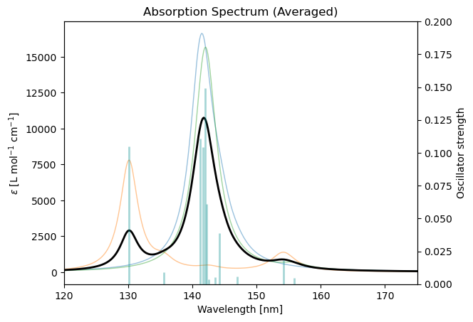
Finally, the averaged spectrum can be plotted:

ens_drv.plot_uv_vis_spectra(
    results,
    show_individual = True,
    show_sticks = True,
    xlim_nm = (150, 275)
)

References¶

Reinholdt, P., Kjellgren, E. R., Steinmann, C., & Olsen, J. M. H. (2020). Cost-Effective Potential for Accurate Polarizable Embedding Calculations in Protein Environments. Journal of Chemical Theory and Computation, 16(2), 1162–1174. 10.1021/acs.jctc.9b00616
Beerepoot, M. T. P., Steindal, A. H., List, N. H., Kongsted, J., & Olsen, J. M. H. (2016). Averaged Solvent Embedding Potential Parameters for Multiscale Modeling of Molecular Properties. Journal of Chemical Theory and Computation, 12(4), 1684–1695. 10.1021/acs.jctc.5b01000
Tian, C., Kasavajhala, K., Belfon, K. A. A., Raguette, L., Huang, H., Migues, A. N., Bickel, J., Wang, Y., Pincay, J., Wu, Q., & Simmerling, C. (2020). ff19SB: Amino-Acid-Specific Protein Backbone Parameters Trained against Quantum Mechanics Energy Surfaces in Solution. Journal of Chemical Theory and Computation, 16(1), 528–552. 10.1021/acs.jctc.9b00591
Jorgensen, W. L., Chandrasekhar, J., Madura, J. D., Impey, R. W., & Klein, M. L. (1983). Comparison of simple potential functions for simulating liquid water. The Journal of Chemical Physics, 79(2), 926–935. 10.1063/1.445869