Localized properties#
ESP charges#
Since there is no unique definition for partial charges and no corresponding physical observable, they can be assigned in several ways, such as being derived from the quantum mechanical electrostatic potential
that can be replaced with a potential caused by the partial charges:
The Merz–Kollman scheme minimizes the squared norm difference between these two quantities evaluated on a set of grid points in the solvent-accessible region of the molecule with respect to variations in the partial charges and a constraint of a conservation of the total molecular charge – the grid points are distributed on successive layers of scaled van der Waals surfaces. This measure is referred to as the figure-of-merit
The resulting electrostatic potential (ESP) charges are obtained by solving the equation
where
and
Python script
import veloxchem as vlx
xyz_str = """6
Methanol
H 1.2001 0.0363 0.8431
C 0.7031 0.0083 -0.1305
H 0.9877 0.8943 -0.7114
H 1.0155 -0.8918 -0.6742
O -0.6582 -0.0067 0.1730
H -1.1326 -0.0311 -0.6482
"""
molecule = vlx.Molecule.read_xyz_string(xyz_str)
basis = vlx.MolecularBasis.read(molecule, "6-31G*")
esp_drv = vlx.RespChargesDriver()
esp_drv.equal_charges = "1=3, 1=4"
esp_charges = esp_drv.compute(molecule, basis, "esp")
Download a Python script
type of input file to calculate the ESP charges for the water molecule at the HF/6-31G level of theory.
Text file
@jobs
task: esp charges
@end
@method settings
basis: 6-31G*
@end
@molecule
charge: 0
multiplicity: 1
xyz:
...
@end
Download a text file
type of input file to calculate the ESP charges for the water molecule at the HF/6-31G level of theory.
In both cases, the user can control the number of layers of the molecular surface as well as the surface grid point density in these layers (in units of Å\(^{-2}\)). In the above examples, the recommended default values are employed.
RESP charges#
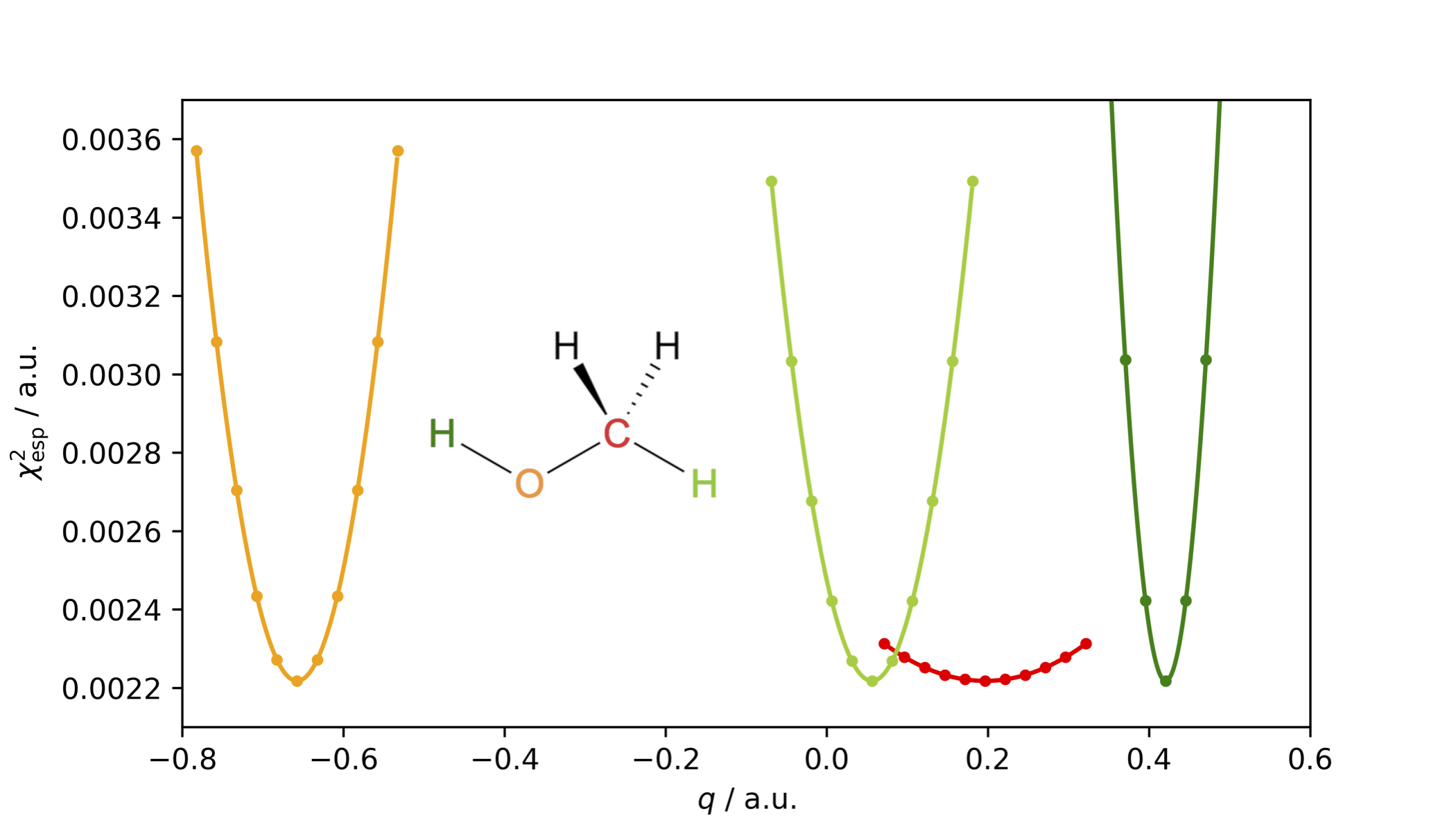
The restrained electrostatic potential (RESP) charge model is an improvement to the Merz–Kollman scheme as the figure-of-merit \(\chi^2_\mathrm{esp}\), is rather insensitive to variations in charges of atoms buried inside the molecule, as illustrated below for methanol and its buried carbon atom in red.

To avoid unphysically large charges of interior atoms, a hyperbolic penalty function is added
so that the diagonal matrix elements become equal to
with a dependency on the partial charge. Consequently, RESP charges are obtained by solving the matrix equation iteratively until the charges and Lagrange multipliers become self-consistent. In addition to that, the RESP charge model allows for the introduction of constraints on charges of equivalent atoms due to symmetry operations or bond rotations.
Python script
import veloxchem as vlx
xyz_str = """6
Methanol
H 1.2001 0.0363 0.8431
C 0.7031 0.0083 -0.1305
H 0.9877 0.8943 -0.7114
H 1.0155 -0.8918 -0.6742
O -0.6582 -0.0067 0.1730
H -1.1326 -0.0311 -0.6482
"""
molecule = vlx.Molecule.read_xyz_string(xyz_str)
basis = vlx.MolecularBasis.read(molecule, "6-31G*")
resp_drv = vlx.RespChargesDriver()
resp_drv.equal_charges = "1=3, 1=4"
resp_charges = resp_drv.compute(molecule, basis, "resp")
Download a Python script
type of input file to calculate the RESP charges for the water molecule at the HF/6-31G* level of theory.
Text file
@jobs
task: resp charges
@end
@method settings
basis: 6-31g*
@end
@resp charges
equal charges: 2 = 3 ! with reference to the atom ordering below
@end
@molecule
charge: 0
multiplicity: 1
xyz:
...
@end
Download a text file
type of input file to calculate the RESP charges for the water molecule at the HF/6-31G* level of theory.
Boltzmann-weighted RESP charges#
If is also possible to calculate the Boltzmann-weighted RESP charges for a set of conformers. In this example, we create three conformers of propanol:
Python script
import veloxchem as vlx
xyz_str = """12
propanol
C 0.287122604482 -0.658439248096 1.352543198101
C 0.224057122961 -0.230177036308 -0.123498537286
C -1.211810163746 -0.086289617161 -0.646362355309
O -1.865244099222 0.943810244897 0.043408964407
H -0.138850281128 0.127254486586 2.013590563967
H 1.345443988487 -0.818617209367 1.650405684477
H -0.266954871175 -1.608743753962 1.513003144654
H 0.758475938136 0.738103480182 -0.253354377301
H 0.752941954799 -0.990737769186 -0.740193839208
H -1.190106706453 0.157165363176 -1.734264017680
H -1.766243401522 -1.044101824780 -0.510744786230
H -1.823078650351 0.710040930866 1.007688030780
"""
molecule = vlx.Molecule.read_xyz_string(xyz_str)
molecule.show(atom_indices=True)
conf = vlx.ConformerGenerator()
conformers = conf.generate(molecule)
3Dmol.js failed to load for some reason. Please check your browser console for error messages.
Self Consistent Field Driver Setup
====================================
Wave Function Model : Spin-Restricted Hartree-Fock
Initial Guess Model : Superposition of Atomic Densities
Convergence Accelerator : Two Level Direct Inversion of Iterative Subspace
Max. Number of Iterations : 50
Max. Number of Error Vectors : 10
Convergence Threshold : 1.0e-06
ERI Screening Threshold : 1.0e-12
Linear Dependence Threshold : 1.0e-06
* Info * Nuclear repulsion energy: 132.6347284236 a.u.
* Info * Overlap matrix computed in 0.00 sec.
* Info * Kinetic energy matrix computed in 0.00 sec.
* Info * Nuclear potential matrix computed in 0.00 sec.
* Info * Orthogonalization matrix computed in 0.00 sec.
* Info * Starting Reduced Basis SCF calculation...
* Info * ...done. SCF energy in reduced basis set: -193.021527086482 a.u. Time: 0.32 sec.
* Info * Overlap matrix computed in 0.00 sec.
* Info * Kinetic energy matrix computed in 0.00 sec.
* Info * Nuclear potential matrix computed in 0.00 sec.
* Info * Orthogonalization matrix computed in 0.00 sec.
Iter. | Hartree-Fock Energy | Energy Change | Gradient Norm | Max. Gradient | Density Change
--------------------------------------------------------------------------------------------
1 -193.098431758322 0.0000000000 0.14187051 0.00778246 0.00000000
2 -193.100823079943 -0.0023913216 0.03993110 0.00294431 0.04766239
3 -193.100998015905 -0.0001749360 0.00977301 0.00063834 0.01267100
4 -193.101012941819 -0.0000149259 0.00276396 0.00022975 0.00419431
5 -193.101014104448 -0.0000011626 0.00093639 0.00007736 0.00153831
6 -193.101014204411 -0.0000001000 0.00020660 0.00001682 0.00030677
7 -193.101014212911 -0.0000000085 0.00004464 0.00000272 0.00013135
8 -193.101014213359 -0.0000000004 0.00001170 0.00000090 0.00002775
9 -193.101014213389 -0.0000000000 0.00000368 0.00000027 0.00000735
10 -193.101014213392 -0.0000000000 0.00000082 0.00000006 0.00000184
*** SCF converged in 10 iterations. Time: 0.96 sec.
Spin-Restricted Hartree-Fock:
-----------------------------
Total Energy : -193.1010142134 a.u.
Electronic Energy : -325.7357426370 a.u.
Nuclear Repulsion Energy : 132.6347284236 a.u.
------------------------------------
Gradient Norm : 0.0000008232 a.u.
Ground State Information
------------------------
Charge of Molecule : 0.0
Multiplicity (2S+1) : 1
Magnetic Quantum Number (M_S) : 0.0
Spin Restricted Orbitals
------------------------
Molecular Orbital No. 13:
--------------------------
Occupation: 2.000 Energy: -0.53973 a.u.
( 1 C 1p+1: 0.29) ( 1 C 1p-1: -0.17) ( 1 C 2p+1: 0.16)
( 4 O 1p+1: 0.28) ( 4 O 1p0 : 0.16) ( 4 O 2p+1: 0.20)
( 6 H 1s : 0.21) ( 6 H 2s : 0.18)
Molecular Orbital No. 14:
--------------------------
Occupation: 2.000 Energy: -0.50615 a.u.
( 1 C 1p+1: -0.17) ( 1 C 1p0 : 0.22) ( 2 C 1p+1: 0.16)
( 2 C 1p0 : -0.23) ( 4 O 1p-1: -0.29) ( 4 O 2p-1: -0.22)
( 7 H 1s : 0.15)
Molecular Orbital No. 15:
--------------------------
Occupation: 2.000 Energy: -0.48962 a.u.
( 1 C 1p-1: 0.21) ( 1 C 1p0 : 0.18) ( 2 C 1p-1: -0.26)
( 2 C 1p0 : -0.19) ( 2 C 2p-1: -0.17) ( 5 H 1s : 0.18)
( 5 H 2s : 0.18) ( 8 H 1s : -0.16) ( 9 H 1s : 0.20)
( 9 H 2s : 0.19)
Molecular Orbital No. 16:
--------------------------
Occupation: 2.000 Energy: -0.46579 a.u.
( 1 C 1p0 : 0.20) ( 2 C 1p-1: 0.16) ( 2 C 1p0 : -0.17)
( 3 C 1p-1: -0.21) ( 3 C 1p0 : 0.22) ( 4 O 1p-1: 0.24)
( 4 O 2p-1: 0.20) ( 10 H 1s : -0.19) ( 10 H 2s : -0.19)
Molecular Orbital No. 17:
--------------------------
Occupation: 2.000 Energy: -0.42749 a.u.
( 2 C 1p+1: 0.27) ( 3 C 1p+1: -0.25) ( 4 O 1p+1: 0.43)
( 4 O 1p-1: 0.20) ( 4 O 2p+1: 0.37) ( 4 O 2p-1: 0.16)
( 11 H 1s : 0.16) ( 11 H 2s : 0.18)
Molecular Orbital No. 18:
--------------------------
Occupation: 0.000 Energy: 0.21031 a.u.
( 1 C 3s : 1.39) ( 1 C 2p0 : 0.40) ( 2 C 3s : 0.47)
( 2 C 2p+1: 0.17) ( 3 C 3s : 0.38) ( 3 C 2p-1: -0.33)
( 4 O 3s : 0.64) ( 4 O 1p0 : 0.17) ( 4 O 2p0 : 0.35)
( 5 H 2s : -0.76) ( 6 H 2s : -0.70) ( 7 H 2s : -0.50)
( 8 H 2s : -0.34) ( 9 H 2s : -0.32) ( 10 H 2s : -0.16)
( 11 H 2s : -0.44) ( 12 H 2s : -0.89)
Molecular Orbital No. 19:
--------------------------
Occupation: 0.000 Energy: 0.25360 a.u.
( 1 C 2p-1: -0.59) ( 2 C 3s : 1.32) ( 2 C 2p+1: 0.39)
( 3 C 3s : 1.08) ( 3 C 2p+1: -0.27) ( 3 C 2p0 : -0.45)
( 4 O 3s : -0.49) ( 5 H 2s : 0.58) ( 6 H 2s : -0.39)
( 7 H 2s : -0.48) ( 8 H 2s : -0.54) ( 9 H 2s : -0.99)
( 10 H 2s : -1.05) ( 11 H 2s : -0.50) ( 12 H 2s : 0.62)
Molecular Orbital No. 20:
--------------------------
Occupation: 0.000 Energy: 0.28223 a.u.
( 1 C 3s : -0.33) ( 1 C 1p-1: 0.15) ( 1 C 2p+1: 0.57)
( 1 C 2p-1: 0.50) ( 2 C 3s : 1.02) ( 2 C 2p-1: 0.36)
( 3 C 3s : -0.81) ( 3 C 1p-1: 0.17) ( 3 C 2p+1: 0.22)
( 3 C 2p-1: 0.53) ( 3 C 2p0 : -0.34) ( 5 H 2s : -0.19)
( 6 H 2s : -0.57) ( 7 H 2s : 1.14) ( 8 H 2s : -1.14)
( 10 H 2s : -0.33) ( 11 H 2s : 1.20)
Molecular Orbital No. 21:
--------------------------
Occupation: 0.000 Energy: 0.28721 a.u.
( 1 C 3s : 1.63) ( 1 C 2p+1: -0.60) ( 1 C 2p-1: -0.25)
( 2 C 3s : 0.49) ( 2 C 2p-1: 0.44) ( 2 C 2p0 : -0.54)
( 3 C 3s : -0.95) ( 3 C 2p+1: -0.28) ( 3 C 2p-1: 0.34)
( 3 C 2p0 : 0.50) ( 4 O 3s : -0.55) ( 4 O 2p-1: 0.17)
( 5 H 2s : -0.84) ( 7 H 2s : -1.21) ( 8 H 2s : -0.72)
( 10 H 2s : 0.75) ( 11 H 2s : 0.57) ( 12 H 2s : 0.51)
Molecular Orbital No. 22:
--------------------------
Occupation: 0.000 Energy: 0.30358 a.u.
( 1 C 3s : 1.23) ( 1 C 1p+1: 0.18) ( 1 C 2p+1: 0.88)
( 1 C 2p-1: -0.29) ( 1 C 2p0 : -0.26) ( 2 C 3s : -0.74)
( 2 C 2p+1: -0.56) ( 2 C 2p-1: -0.56) ( 2 C 2p0 : -0.41)
( 3 C 3s : -1.14) ( 3 C 2p+1: 0.22) ( 3 C 2p-1: 0.35)
( 5 H 2s : 0.52) ( 6 H 2s : -1.45) ( 7 H 2s : -0.36)
( 8 H 2s : 1.08) ( 9 H 2s : -0.32) ( 10 H 2s : 0.30)
( 11 H 2s : 0.85)
Ground State Dipole Moment
----------------------------
X : 0.393044 a.u. 0.999019 Debye
Y : -0.576142 a.u. -1.464406 Debye
Z : 0.305368 a.u. 0.776167 Debye
Total : 0.761362 a.u. 1.935190 Debye
RESP Charges Driver Setup
===========================
Number of Conformers : 1
Number of Layers : 4
Points per Square Angstrom : 1.0
Total Number of Grid Points : 625
First Stage Fit
-----------------
Restraint Strength : 0.0005
Restrained Hydrogens : No
Max. Number of Iterations : 50
Convergence Threshold (a.u.) : 1e-06
*** Charge fitting converged in 10 iterations.
No. | Atom | Constraints | Charges (a.u.)
--------------------------------------------
1 C -0.113903
2 C 0.019214
3 C 0.125225
4 O -0.630091
5 H 0.018365
6 H 0.036674
7 H 0.035046
8 H 0.029194
9 H -0.010010
10 H 0.069240
11 H 0.015389
12 H 0.405656
--------------------------------------------
Total Charge : 0.000000
Fit Quality
-------------
Relative Root-Mean-Square Error : 0.152960
Second Stage Fit
------------------
Restraint Strength : 0.001
Restrained Hydrogens : No
Max. Number of Iterations : 50
Convergence Threshold (a.u.) : 1e-06
*** Charge fitting converged in 12 iterations.
No. | Atom | Frozen | Constraints | Charges (a.u.)
----------------------------------------------------
1 C No -0.170274
2 C No -0.024649
3 C No 0.173472
4 O Yes -0.630091
5 H No 0.043005
6 H No 5 0.043005
7 H No 6 0.043005
8 H No 0.033351
9 H No 8 0.033351
10 H No 0.025084
11 H No 10 0.025084
12 H Yes 0.405656
----------------------------------------------------
Total Charge : 0.000000
Fit Quality
-------------
Relative Root-Mean-Square Error : 0.192291
Reference:
J. Phys. Chem. 1993, 97, 10269-10280.
* Info * 9 conformers will be generated.
* Info * 9 conformers generated in 0.01 sec
* Info * Energy minimization of 9 conformers took 0.07 sec
* Info * Global minimum energy: 14.609 kJ/mol
* Info * 3 conformers remain after removal of duplicate conformers.
* Info * Total time spent in generating conformers: 1.60 sec
conf.show_conformers(number=3, atom_indices=True)
Conformer 1 with energy 14.609 kJ/mol
3Dmol.js failed to load for some reason. Please check your browser console for error messages.
Conformer 2 with energy 17.583 kJ/mol
3Dmol.js failed to load for some reason. Please check your browser console for error messages.
Conformer 3 with energy 17.765 kJ/mol
3Dmol.js failed to load for some reason. Please check your browser console for error messages.
# Now we will compute the Boltzmann-weighted RESP charges:
empty_mol = vlx.Molecule()
empty_bas = vlx.MolecularBasis()
resp_settings = {
'molecules': conformers['molecules'],
'filename': 'resp'
}
method_settings = {'basis': '6-31g*'}
resp_drv = vlx.RespChargesDriver()
resp_drv.update_settings(resp_settings, method_settings)
resp_charges = resp_drv.compute(empty_mol, empty_bas, 'resp')
print("Boltzmann-weighted RESP charges =" , resp_charges)
* Info * Found 3 conformers from molecule list.
* Info * Processing conformer 1...
Molecular Geometry (Angstroms)
================================
Atom Coordinate X Coordinate Y Coordinate Z
C 0.293102854750 -0.675770240189 1.367361895492
C 0.206109191925 -0.221436473583 -0.109150294181
C -1.229333228297 -0.092535333874 -0.658192410832
O -1.940179948964 0.878365794385 0.063157279904
H -0.134335471512 0.085226397053 2.056076726749
H 1.358594029910 -0.817615151195 1.650115065577
H -0.232799807931 -1.643603948768 1.521281220543
H 0.733940227753 0.751914775944 -0.234435084863
H 0.746175323299 -0.966156879303 -0.736092261274
H -1.191925654625 0.206263258528 -1.732337850704
H -1.754096696203 -1.074640404572 -0.590250455068
H -1.822990234848 0.652477282621 1.023697867396
Molecular charge : 0
Spin multiplicity : 1
Number of atoms : 12
Number of alpha electrons : 17
Number of beta electrons : 17
Molecular Basis (Atomic Basis)
================================
Basis: 6-31G*
Atom Contracted GTOs Primitive GTOs
C (3S,2P,1D) (10S,4P,1D)
O (3S,2P,1D) (10S,4P,1D)
H (2S) (4S)
Contracted Basis Functions : 72
Primitive Basis Functions : 140
* Info * Processing conformer 2...
Molecular Geometry (Angstroms)
================================
Atom Coordinate X Coordinate Y Coordinate Z
C 0.283461903383 -0.633328769933 1.355989801141
C 0.204307971591 -0.224076341405 -0.133112169370
C -1.229192131799 -0.085087870589 -0.688136844353
O -1.930123923283 0.917680887775 0.000884082996
H -0.163786873091 0.141428167979 2.016494795373
H 1.346584568792 -0.756955175357 1.655173008689
H -0.237472873378 -1.599985574897 1.532303249308
H 0.753318379941 0.732750619892 -0.288861180036
H 0.729553246983 -0.999532832827 -0.734932154363
H -1.179817010386 0.183516335978 -1.769729198116
H -1.772707358915 -1.055182576731 -0.598392956756
H -1.271814444252 1.627975583921 0.221400977732
Molecular charge : 0
Spin multiplicity : 1
Number of atoms : 12
Number of alpha electrons : 17
Number of beta electrons : 17
Molecular Basis (Atomic Basis)
================================
Basis: 6-31G*
Atom Contracted GTOs Primitive GTOs
C (3S,2P,1D) (10S,4P,1D)
O (3S,2P,1D) (10S,4P,1D)
H (2S) (4S)
Contracted Basis Functions : 72
Primitive Basis Functions : 140
* Info * Processing conformer 3...
Molecular Geometry (Angstroms)
================================
Atom Coordinate X Coordinate Y Coordinate Z
C 0.286309558593 -0.690270263577 1.340939142000
C 0.210012018563 -0.242974882210 -0.137527916929
C -1.221764176641 -0.052555704695 -0.682495024078
O -1.942880831335 -1.255315976563 -0.610151277492
H -0.217540055587 0.043088373394 2.008099096708
H 1.349310674037 -0.759276543921 1.657598940522
H -0.179834340555 -1.689118199210 1.488087821239
H 0.757312060893 0.720654906669 -0.250573700752
H 0.739133366571 -0.990933928355 -0.770139461113
H -1.750568036714 0.727393008087 -0.085310921565
H -1.177965965409 0.295291085728 -1.741479166764
H -1.304751077784 -1.985772377366 -0.823941972090
Molecular charge : 0
Spin multiplicity : 1
Number of atoms : 12
Number of alpha electrons : 17
Number of beta electrons : 17
Molecular Basis (Atomic Basis)
================================
Basis: 6-31G*
Atom Contracted GTOs Primitive GTOs
C (3S,2P,1D) (10S,4P,1D)
O (3S,2P,1D) (10S,4P,1D)
H (2S) (4S)
Contracted Basis Functions : 72
Primitive Basis Functions : 140
RESP Charges Driver Setup
===========================
Number of Conformers : 3
Weights of Conformers : 0.266385
0.288254
0.445361
Number of Layers : 4
Points per Square Angstrom : 1.0
Total Number of Grid Points : 1852
First Stage Fit
-----------------
Restraint Strength : 0.0005
Restrained Hydrogens : No
Max. Number of Iterations : 50
Convergence Threshold (a.u.) : 1e-06
*** Charge fitting converged in 10 iterations.
No. | Atom | Constraints | Charges (a.u.)
--------------------------------------------
1 C -0.047037
2 C 0.030736
3 C 0.156881
4 O -0.612997
5 H 0.017208
6 H 0.008562
7 H 0.019074
8 H -0.005458
9 H -0.008223
10 H 0.042932
11 H 0.017688
12 H 0.380634
--------------------------------------------
Total Charge : 0.000000
Fit Quality
-------------
Relative Root-Mean-Square Error : 0.184701
Second Stage Fit
------------------
Restraint Strength : 0.001
Restrained Hydrogens : No
Max. Number of Iterations : 50
Convergence Threshold (a.u.) : 1e-06
*** Charge fitting converged in 5 iterations.
No. | Atom | Frozen | Constraints | Charges (a.u.)
----------------------------------------------------
1 C No -0.031030
2 C No 0.030609
3 C No 0.159303
4 O Yes -0.612997
5 H No 0.010376
6 H No 5 0.010376
7 H No 6 0.010376
8 H No -0.009273
9 H No 8 -0.009273
10 H No 0.030450
11 H No 10 0.030450
12 H Yes 0.380634
----------------------------------------------------
Total Charge : 0.000000
Fit Quality
-------------
Relative Root-Mean-Square Error : 0.193735
Reference:
J. Phys. Chem. 1993, 97, 10269-10280.
J. Am. Chem. Soc. 1992, 114, 9075-9079.
Boltzmann-weighted RESP charges = [-0.03103009 0.03060905 0.15930278 -0.61299669 0.01037559 0.01037559
0.01037559 -0.00927313 -0.00927313 0.03045008 0.03045008 0.38063429]
Download a Python script
type of input file to calculate the Boltzmann-weighted RESP charges for the three conformers of propanol at the HF/6-31G* level of theory.
Note that the argument 'filename': 'resp'
instructs the creation of a folder named resp_files
which will contain the SCF output of all conformers.
Alternatively, one can also provide a file containing the XYZ coordinates of all conformers:
resp_settings = {
'xyz_file': 'all_conformers.xyz'
}
Text file
@jobs
task: resp charges
@end
@method settings
basis: 6-31g*
@end
@resp charges
xyz_file: all_conformers.xyz
@end
@molecule
charge: 0
multiplicity: 1
@end
Download a text file
type of input file to calculate the Boltzmann-weighted RESP charges for the three conformers of propanol at the HF/6-31G* level of theory, and use the all_conformers.xyz
file.
CHELPG charges#
Different choices of grid points in the Merz–Kollman (MK) scheme can be made. CHELPG charges are obtained with grid points chosen on a dense cubic grid with exclusion made of grid points inside the van der Waals molecular volume.
In contrast to the original MK scheme, the calculation of CHELPG charges involve grid points directly outside the van der Waals molecular volume, and since the electrostatic potential is here large, these points will be important for the minimization of the Lagrangian. We note that there is no universal grid-point choice that can be considered best for all situations.
Python script
import veloxchem as vlx
xyz_str = """6
Methanol
H 1.2001 0.0363 0.8431
C 0.7031 0.0083 -0.1305
H 0.9877 0.8943 -0.7114
H 1.0155 -0.8918 -0.6742
O -0.6582 -0.0067 0.1730
H -1.1326 -0.0311 -0.6482
"""
molecule = vlx.Molecule.read_xyz_string(xyz_str)
basis = vlx.MolecularBasis.read(molecule, "6-31G*")
esp_drv = vlx.RespChargesDriver()
esp_drv.grid_type = "chelpg"
esp_drv.equal_charges = "1=3, 1=4"
chelpg_charges = esp_drv.compute(molecule, basis, "esp")
Charge comparison#
The localized charges for methanol in the examples above become:
Atom ESP charge RESP charge CHELPG charge
--------------------------------------------------------
H 0.023220 -0.031030 0.003200
C 0.148458 0.030609 0.225480
H 0.023220 0.159303 0.003200
H 0.023220 -0.612997 0.003200
O -0.594785 0.010376 -0.611345
H 0.376669 0.010376 0.376265
--------------------------------------------------------
Total: 0.000000 0.000000 -0.000000
LoProp charges and polarizabilities#
The LoProp approach [GLKarlstrom04] is implemented for the determination of localized (atomic) charges and polarizabilities that enter into polarizable embedding calculations of optical spectra.
Python script
import veloxchem as vlx
molecule = vlx.Molecule.read_molecule_string(
"""
O 0.0000000 0.0000000 -0.1653507
H 0.7493682 0.0000000 0.4424329
H -0.7493682 0.0000000 0.4424329
"""
)
basis = vlx.MolecularBasis.read(molecule, "ANO-S-VDZP")
scf_drv = vlx.ScfRestrictedDriver()
scf_results = scf_drv.compute(molecule, basis)
loprop_drv = vlx.PEForceFieldGenerator()
loprop_results = loprop_drv.compute(molecule, basis, scf_results)
This calculation gives the following results.
LoProp charges (a.u.):
O: -0.6777
H: 0.3388
H: 0.3388
LoProp polarizabilities (a.u.):
xx yy zz
O: 3.88 2.91 3.69
H: 1.84 1.21 1.57
H: 1.84 1.21 1.57
Download a Python script
type of input file to calculate the LOPROP charges and atomic polarizabilities for the water molecule at the B3LYP/ANO-S-VDPZ level of theory.
Text file
@jobs
task: loprop
@end
@method settings
xcfun: b3lyp
basis: ANO-S-VDZP ! An ANO type of basis set should be used
@end
@molecule
charge: 0
multiplicity: 1
xyz:
...
@end
Download a text file
the input file to calculate the LoProp charges and atomic polarizabilities for the water molecule at the B3LYP/ANO-S-VDPZ level of theory.
