Jupyter notebooks#
Here, we explain how to visualize VeloxChem results in Jupyter notebooks.
The underlying calculation can be obtained either directly in a notebook or imported from a VeloxChem .h5 file.
import veloxchem as vlx
Molecular structure#
In Jupyter notebook, a molecule object can be visualized using the show function.
The atom_indices and atom_labels options can be used.
From a notebook cell
molecule = vlx.Molecule.read_smiles('C1=CC=C(C=C1)C(=O)O')

molecule.show(atom_indices=True, atom_labels=True)
3Dmol.js failed to load for some reason. Please check your browser console for error messages.
From an h5 file
biph_dict = vlx.read_results("../output_files/biphenyl-scf.h5", label="scf")
biph = vlx.Molecule.from_dict(biph_dict)

biph.show()
3Dmol.js failed to load for some reason. Please check your browser console for error messages.
Structure optimization#
From notebook cell
molecule = vlx.Molecule.read_smiles('CCO')
basis = vlx.MolecularBasis.read(molecule, 'def2-svp')

scf_drv = vlx.ScfRestrictedDriver()
scf_drv.xcfun = 'b3lyp'
results = scf_drv.compute(molecule, basis)

opt_drv = vlx.OptimizationDriver(scf_drv)
opt_results = opt_drv.compute(molecule, basis, results)
opt_drv.show_convergence(opt_results)
From an h5 file
opt_results = vlx.read_results("../output_files/bithio-S0-opt.h5", label="opt")
opt_drv.show_convergence(opt_results)
Spectrum plotting#
From a notebook cell
molecule = vlx.Molecule.read_smiles('CCO')
basis = vlx.MolecularBasis.read(molecule, 'def2-svp')

scf_drv = vlx.ScfRestrictedDriver()
scf_drv.xcfun = 'b3lyp'
scf_results = scf_drv.compute(molecule, basis)

rsp_drv = vlx.lreigensolver.LinearResponseEigenSolver()
rsp_drv.nstates = 10
rsp_results = rsp_drv.compute(molecule, basis, scf_results)
rsp_drv.plot(rsp_results)
From an h5 file
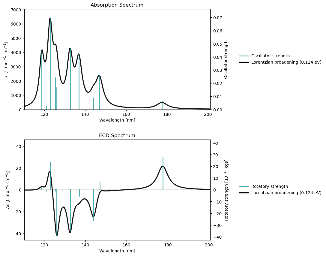
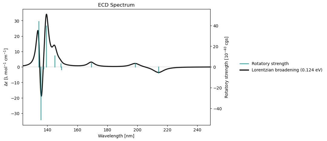
rsp_results = vlx.read_results("../output_files/alanine-ecd.h5", label="rsp")
rsp_drv.plot_ecd(rsp_results)
Normal modes#
From a notebook cell
molecule = vlx.Molecule.read_smiles('CCO')
basis = vlx.MolecularBasis.read(molecule, 'def2-svp')

scf_drv = vlx.ScfRestrictedDriver()
scf_drv.xcfun = 'b3lyp'
scf_results = scf_drv.compute(molecule, basis)

vib_drv = vlx.VibrationalAnalysis(scf_drv)
vib_results = vib_drv.compute(molecule, basis)
vib_drv.plot(vib_results)
vib_drv.animate(vib_results, mode=14)
3Dmol.js failed to load for some reason. Please check your browser console for error messages.
From an h5 file
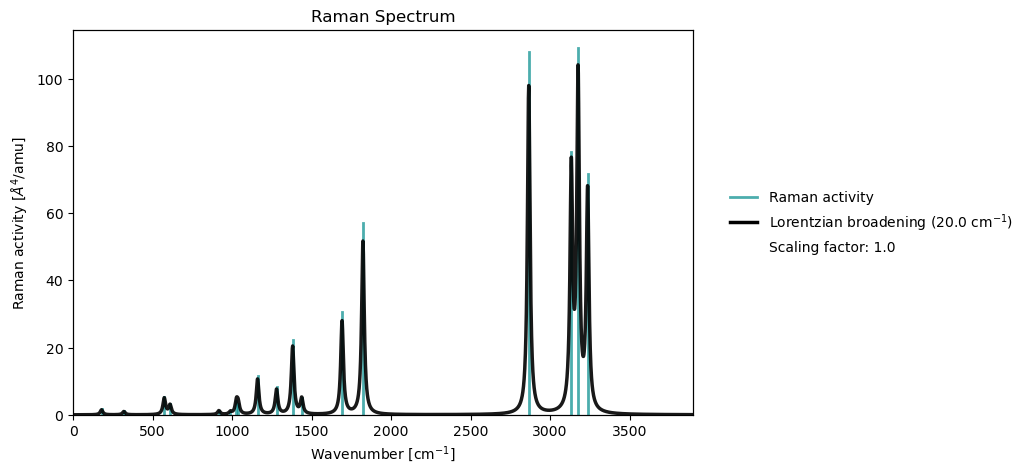
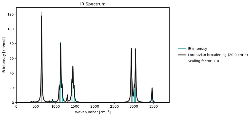
vib_results = vlx.read_results("../output_files/acro-raman.h5", label="vib")
vib_drv.plot_raman(vib_results)
vib_drv.animate(vib_results, mode=14)
3Dmol.js failed to load for some reason. Please check your browser console for error messages.