ESP charges
Since there is no unique definition for partial charges and no corresponding physical observable, they can be assigned in several ways, such as being derived from the quantum mechanical electrostatic potential
that can be replaced with a potential caused by the partial charges:
The Merz–Kollman scheme minimizes the squared norm difference between these two quantities evaluated on a set of grid points in the solvent-accessible region of the molecule with respect to variations in the partial charges and a constraint of a conservation of the total molecular charge – the grid points are distributed on successive layers of scaled van der Waals surfaces. This measure is referred to as the figure-of-merit
The resulting electrostatic potential (ESP) charges are obtained by solving the equation
where
and
Python script
import veloxchem as vlx

xyz_str = """6
Methanol
H      1.2001      0.0363      0.8431
C      0.7031      0.0083     -0.1305
H      0.9877      0.8943     -0.7114
H      1.0155     -0.8918     -0.6742
O     -0.6582     -0.0067      0.1730
H     -1.1326     -0.0311     -0.6482
"""

molecule = vlx.Molecule.read_xyz_string(xyz_str)
basis = vlx.MolecularBasis.read(molecule, "6-31G*")

esp_drv = vlx.EspChargesDriver()
esp_drv.equal_charges = "1=3, 1=4"
esp_charges = esp_drv.compute(molecule, basis)
                                            Self Consistent Field Driver Setup
                                           ====================================

                   Wave Function Model             : Spin-Restricted Hartree-Fock
                   Initial Guess Model             : Superposition of Atomic Densities
                   Convergence Accelerator         : Two Level Direct Inversion of Iterative Subspace
                   Max. Number of Iterations       : 50
                   Max. Number of Error Vectors    : 10
                   Convergence Threshold           : 1.0e-06
                   ERI Screening Threshold         : 1.0e-12
                   Linear Dependence Threshold     : 1.0e-06

* Info * Starting Reduced Basis SCF calculation...
* Info * ...done. SCF energy in reduced basis set: -114.985032880309 a.u. Time: 0.04 sec.


               Iter. | Hartree-Fock Energy | Energy Change | Gradient Norm | Max. Gradient | Density Change
               --------------------------------------------------------------------------------------------
                  1      -115.032021654336    0.0000000000      0.10560685      0.01073554      0.00000000
                  2      -115.033365303353   -0.0013436490      0.02909872      0.00322626      0.03152624
                  3      -115.033457176280   -0.0000918729      0.00644690      0.00095115      0.00787787
                  4      -115.033464315327   -0.0000071390      0.00211836      0.00024088      0.00282760
                  5      -115.033465123955   -0.0000008086      0.00065282      0.00008165      0.00126450
                  6      -115.033465189352   -0.0000000654      0.00017067      0.00002207      0.00027179
                  7      -115.033465196949   -0.0000000076      0.00003215      0.00000409      0.00012239
                  8      -115.033465197230   -0.0000000003      0.00000526      0.00000072      0.00002194
                  9      -115.033465197239   -0.0000000000      0.00000118      0.00000014      0.00000427
                 10      -115.033465197239   -0.0000000000      0.00000018      0.00000002      0.00000090

               *** SCF converged in 10 iterations. Time: 0.10 sec.

               Spin-Restricted Hartree-Fock:
               -----------------------------
               Total Energy                       :     -115.0334651972 a.u.
               Electronic Energy                  :     -155.8239921029 a.u.
               Nuclear Repulsion Energy           :       40.7905269056 a.u.
               ------------------------------------
               Gradient Norm                      :        0.0000001843 a.u.


               Ground State Information
               ------------------------
               Charge of Molecule            :  0.0
               Multiplicity (2S+1)           :  1
               Magnetic Quantum Number (M_S) :  0.0


                                                RESP Charges Driver Setup
                                               ===========================

                                         Number of Conformers         :  1
                                         Number of Layers             :  4
                                         Points per Square Angstrom   :  1.0
                                         Total Number of Grid Points  :  420

                                                 Merz-Kollman ESP Charges
                                                --------------------------

                                              No.   Atom      Charge (a.u.)
                                             -------------------------------
                                                1     H         0.023220
                                                2     C         0.148458
                                                3     H         0.023220
                                                4     H         0.023220
                                                5     O        -0.594785
                                                6     H         0.376669
                                             -------------------------------
                                               Total Charge  :  0.000000

                                                       Fit Quality
                                                      -------------
                                       Relative Root-Mean-Square Error  :  0.180034

                                       Reference:
                                       J. Comput. Chem. 1984, 5, 129-145.
Text file
@jobs
task: esp charges
@end

@method settings
basis: 6-31G*
@end

@molecule
charge: 0
multiplicity: 1
xyz:
...
@end
In both cases, the user can control the number of layers of the molecular surface as well as the surface grid point density in these layers (in units of Å−2). In the above examples, the recommended default values are employed.
RESP charges
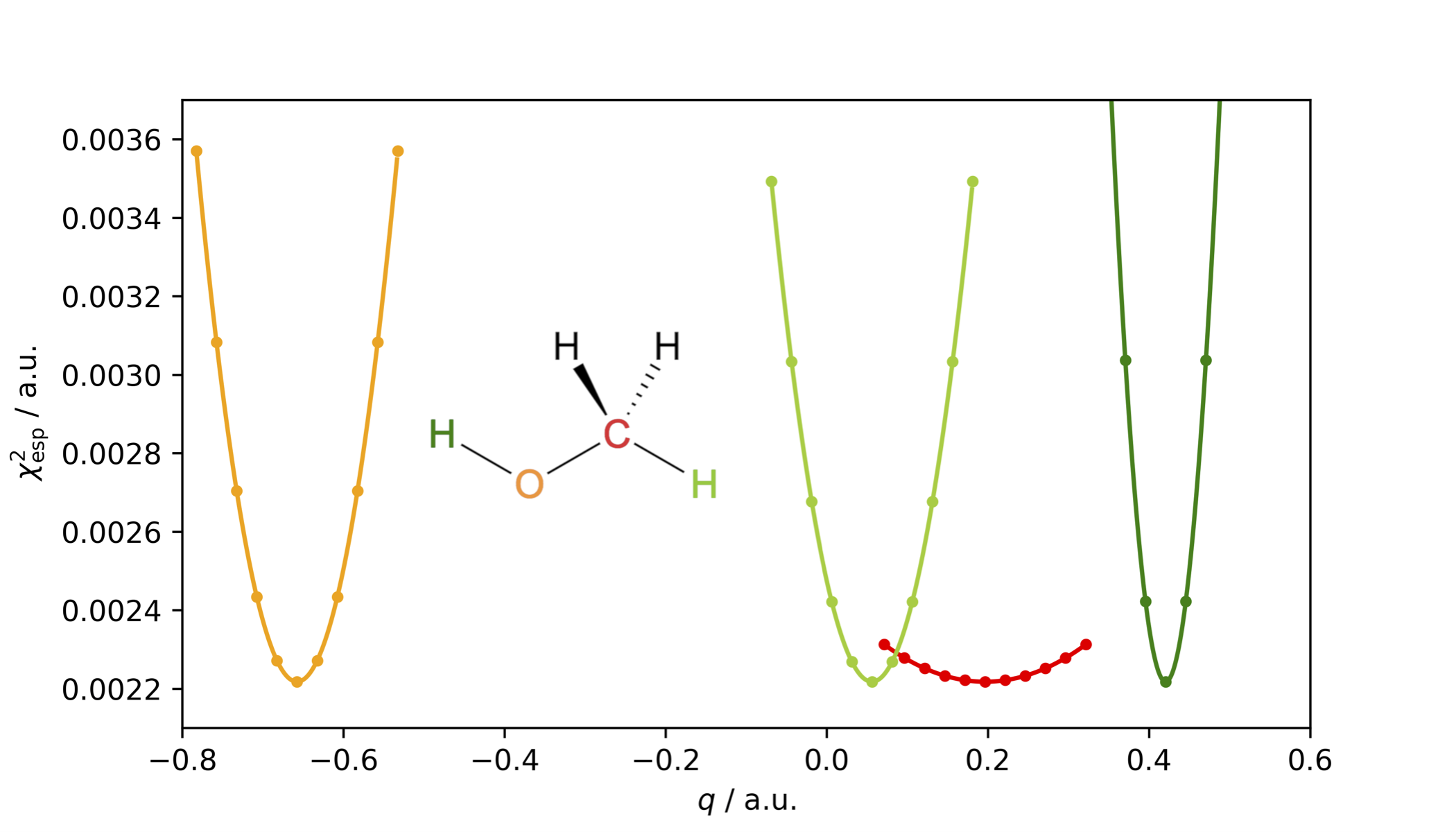
The restrained electrostatic potential (RESP) charge model is an improvement to the Merz–Kollman scheme as the figure-of-merit χesp2, is rather insensitive to variations in charges of atoms buried inside the molecule, as illustrated below for methanol and its buried carbon atom in red.
To avoid unphysically large charges of interior atoms, a hyperbolic penalty function is added
so that the diagonal matrix elements become equal to
with a dependency on the partial charge. Consequently, RESP charges are obtained by solving the matrix equation iteratively until the charges and Lagrange multipliers become self-consistent. In addition to that, the RESP charge model allows for the introduction of constraints on charges of equivalent atoms due to symmetry operations or bond rotations.
Python script
import veloxchem as vlx

xyz_str = """6
Methanol
H      1.2001      0.0363      0.8431
C      0.7031      0.0083     -0.1305
H      0.9877      0.8943     -0.7114
H      1.0155     -0.8918     -0.6742
O     -0.6582     -0.0067      0.1730
H     -1.1326     -0.0311     -0.6482
"""

molecule = vlx.Molecule.read_xyz_string(xyz_str)
basis = vlx.MolecularBasis.read(molecule, "6-31G*")

resp_drv = vlx.RespChargesDriver()
resp_drv.equal_charges = "1=3, 1=4"
resp_charges = resp_drv.compute(molecule, basis)
                                            Self Consistent Field Driver Setup
                                           ====================================

                   Wave Function Model             : Spin-Restricted Hartree-Fock
                   Initial Guess Model             : Superposition of Atomic Densities
                   Convergence Accelerator         : Two Level Direct Inversion of Iterative Subspace
                   Max. Number of Iterations       : 50
                   Max. Number of Error Vectors    : 10
                   Convergence Threshold           : 1.0e-06
                   ERI Screening Threshold         : 1.0e-12
                   Linear Dependence Threshold     : 1.0e-06

* Info * Starting Reduced Basis SCF calculation...
* Info * ...done. SCF energy in reduced basis set: -114.985032880309 a.u. Time: 0.05 sec.


               Iter. | Hartree-Fock Energy | Energy Change | Gradient Norm | Max. Gradient | Density Change
               --------------------------------------------------------------------------------------------
                  1      -115.032021654336    0.0000000000      0.10560685      0.01073554      0.00000000
                  2      -115.033365303353   -0.0013436490      0.02909872      0.00322626      0.03152624
                  3      -115.033457176279   -0.0000918729      0.00644690      0.00095115      0.00787787
                  4      -115.033464315327   -0.0000071390      0.00211836      0.00024088      0.00282760
                  5      -115.033465123956   -0.0000008086      0.00065282      0.00008165      0.00126450
                  6      -115.033465189352   -0.0000000654      0.00017067      0.00002207      0.00027179
                  7      -115.033465196950   -0.0000000076      0.00003215      0.00000409      0.00012239
                  8      -115.033465197230   -0.0000000003      0.00000526      0.00000072      0.00002194
                  9      -115.033465197239   -0.0000000000      0.00000118      0.00000014      0.00000427
                 10      -115.033465197239   -0.0000000000      0.00000018      0.00000002      0.00000090

               *** SCF converged in 10 iterations. Time: 0.12 sec.

               Spin-Restricted Hartree-Fock:
               -----------------------------
               Total Energy                       :     -115.0334651972 a.u.
               Electronic Energy                  :     -155.8239921029 a.u.
               Nuclear Repulsion Energy           :       40.7905269056 a.u.
               ------------------------------------
               Gradient Norm                      :        0.0000001843 a.u.


               Ground State Information
               ------------------------
               Charge of Molecule            :  0.0
               Multiplicity (2S+1)           :  1
               Magnetic Quantum Number (M_S) :  0.0


                                                RESP Charges Driver Setup
                                               ===========================

                                         Number of Conformers         :  1
                                         Number of Layers             :  4
                                         Points per Square Angstrom   :  1.0
                                         Total Number of Grid Points  :  420


                                                     First Stage Fit
                                                    -----------------

                                         Restraint Strength           :  0.0005
                                         Restrained Hydrogens         :  No
                                         Max. Number of Iterations    :  50
                                         Convergence Threshold (a.u.) :  1e-06

                                      *** Charge fitting converged in 9 iterations.

                                        No. | Atom |  Constraints | Charges (a.u.)
                                       --------------------------------------------
                                          1     H                      0.075643
                                          2     C                      0.117258
                                          3     H                      0.013902
                                          4     H                      0.013047
                                          5     O                     -0.639004
                                          6     H                      0.419154
                                       --------------------------------------------
                                               Total Charge  :  0.000000

                                                       Fit Quality
                                                      -------------
                                       Relative Root-Mean-Square Error  :  0.139861


                                                     Second Stage Fit
                                                    ------------------

                                         Restraint Strength           :  0.001
                                         Restrained Hydrogens         :  No
                                         Max. Number of Iterations    :  50
                                         Convergence Threshold (a.u.) :  1e-06

                                      *** Charge fitting converged in 4 iterations.

                                    No. | Atom | Frozen | Constraints | Charges (a.u.)
                                   ----------------------------------------------------
                                      1     H       No                     0.033747
                                      2     C       No                     0.118610
                                      3     H       No         1           0.033747
                                      4     H       No         1           0.033747
                                      5     O      Yes                    -0.639004
                                      6     H      Yes                     0.419154
                                   ----------------------------------------------------
                                               Total Charge  :  0.000000

                                                       Fit Quality
                                                      -------------
                                       Relative Root-Mean-Square Error  :  0.203249

                                       Reference:
                                       J. Phys. Chem. 1993, 97, 10269-10280.
Text file
@jobs
task: resp charges
@end

@method settings
basis: 6-31g*
@end

@resp charges
equal charges: 2 = 3    ! with reference to the atom ordering below
@end

@molecule
charge: 0
multiplicity: 1
xyz:
...
@end
Boltzmann-weighted RESP charges
It is also possible to calculate the Boltzmann-weighted RESP charges for a set of conformers.
Python script
Below, the argument conformers is a list of molecule objects for which the averaging is performed. By default, the calculation is performed at the Hartree–Fock level using the 6-31G* basis set.
import veloxchem as vlx

molecule = vlx.Molecule.read_name("propanol")

confgen = vlx.ConformerGenerator()
conformers = confgen.generate(molecule)

resp_drv = vlx.RespChargesDriver()
resp_charges = resp_drv.compute(conformers["molecules"])
Reading propanol from PubChem...
Reference: S. Kim, J. Chen, T. Cheng, A. Gindulyte, J. He, S. He, Q. Li, B. A. Shoemaker, P. A. Thiessen, B. Yu, L. Zaslavsky, J. Zhang, E. E. Bolton, Nucleic Acids Res., 2025, 53, D1516-D1525.
Please double-check the compound since names may refer to more than one record.
Self Consistent Field Driver Setup
====================================
Wave Function Model : Spin-Restricted Hartree-Fock
Initial Guess Model : Superposition of Atomic Densities
Convergence Accelerator : Two Level Direct Inversion of Iterative Subspace
Max. Number of Iterations : 50
Max. Number of Error Vectors : 10
Convergence Threshold : 1.0e-06
ERI Screening Threshold : 1.0e-12
Linear Dependence Threshold : 1.0e-06
* Info * Starting Reduced Basis SCF calculation...
* Info * ...done. SCF energy in reduced basis set: -193.023573894114 a.u. Time: 0.54 sec.
Iter. | Hartree-Fock Energy | Energy Change | Gradient Norm | Max. Gradient | Density Change
--------------------------------------------------------------------------------------------
1 -193.100552007396 0.0000000000 0.14021258 0.01285532 0.00000000
2 -193.102905969491 -0.0023539621 0.03455805 0.00350330 0.04656359
3 -193.103041674949 -0.0001357055 0.00845048 0.00072688 0.01025461
4 -193.103053346377 -0.0000116714 0.00252513 0.00025412 0.00359815
5 -193.103054502118 -0.0000011557 0.00072805 0.00005845 0.00155264
6 -193.103054578079 -0.0000000760 0.00018260 0.00002441 0.00030255
7 -193.103054585964 -0.0000000079 0.00003985 0.00000334 0.00013504
8 -193.103054586362 -0.0000000004 0.00001242 0.00000118 0.00002528
9 -193.103054586400 -0.0000000000 0.00000318 0.00000036 0.00000837
10 -193.103054586403 -0.0000000000 0.00000068 0.00000008 0.00000255
*** SCF converged in 10 iterations. Time: 1.35 sec.
Spin-Restricted Hartree-Fock:
-----------------------------
Total Energy : -193.1030545864 a.u.
Electronic Energy : -323.2841944409 a.u.
Nuclear Repulsion Energy : 130.1811398545 a.u.
------------------------------------
Gradient Norm : 0.0000006799 a.u.
Ground State Information
------------------------
Charge of Molecule : 0.0
Multiplicity (2S+1) : 1
Magnetic Quantum Number (M_S) : 0.0
RESP Charges Driver Setup
===========================
Number of Conformers : 1
Number of Layers : 4
Points per Square Angstrom : 1.0
Total Number of Grid Points : 630
First Stage Fit
-----------------
Restraint Strength : 0.0005
Restrained Hydrogens : No
Max. Number of Iterations : 50
Convergence Threshold (a.u.) : 1e-06
*** Charge fitting converged in 12 iterations.
No. | Atom | Constraints | Charges (a.u.)
--------------------------------------------
1 C -0.289527
2 C 0.128656
3 C 0.221520
4 O -0.692337
5 H 0.067562
6 H 0.061656
7 H 0.061441
8 H 0.015758
9 H 0.015022
10 H -0.005840
11 H -0.004387
12 H 0.420476
--------------------------------------------
Total Charge : 0.000000
Fit Quality
-------------
Relative Root-Mean-Square Error : 0.117609
Second Stage Fit
------------------
Restraint Strength : 0.001
Restrained Hydrogens : No
Max. Number of Iterations : 50
Convergence Threshold (a.u.) : 1e-06
*** Charge fitting converged in 14 iterations.
No. | Atom | Frozen | Constraints | Charges (a.u.)
----------------------------------------------------
1 C No -0.187792
2 C No 0.071025
3 C No 0.229465
4 O Yes -0.692337
5 H No 0.038646
6 H No 5 0.038646
7 H No 6 0.038646
8 H No 0.027480
9 H No 8 0.027480
10 H No -0.005867
11 H No 10 -0.005867
12 H Yes 0.420476
----------------------------------------------------
Total Charge : 0.000000
Fit Quality
-------------
Relative Root-Mean-Square Error : 0.124633
Reference:
J. Phys. Chem. 1993, 97, 10269-10280.
* Info * 9 conformers will be generated.
* Info * 9 conformers generated in 0.01 sec
* Info * Energy minimization of 9 conformers took 0.03 sec
* Info * Global minimum energy: 24.197 kJ/mol
* Info * 4 conformers remain after removal of duplicate conformers.
* Info * Total time spent in generating conformers: 2.10 sec
* Info * Processing conformer 1...
Molecular Geometry (Angstroms)
================================
Atom Coordinate X Coordinate Y Coordinate Z
C 0.317388580166 1.728759406358 1.143135271318
C 0.653517496979 0.654111189338 0.096911735710
C 0.466925404369 -0.782302477385 0.617234710100
O 1.338179753320 -1.038546906374 1.686796347289
H 0.400197335426 2.734112299159 0.678250793072
H -0.721665765587 1.602093200563 1.516681797808
H 1.024588257933 1.686009163406 1.999141790031
H -0.010352238938 0.799812548842 -0.783204732407
H 1.703246282797 0.789793605779 -0.245259127934
H 0.677959583715 -1.500796100373 -0.206702800607
H -0.584786742746 -0.924718913758 0.954171949434
H 1.058826555931 -0.426944203649 2.417562511082
Molecular charge : 0
Spin multiplicity : 1
Number of atoms : 12
Number of alpha electrons : 17
Number of beta electrons : 17
Molecular Basis (Atomic Basis)
================================
Basis: 6-31G*
Atom Contracted GTOs Primitive GTOs
C (3S,2P,1D) (10S,4P,1D)
O (3S,2P,1D) (10S,4P,1D)
H (2S) (4S)
Contracted Basis Functions : 72
Primitive Basis Functions : 140
Self Consistent Field Driver Setup
====================================
Wave Function Model : Spin-Restricted Hartree-Fock
Initial Guess Model : Superposition of Atomic Densities
Convergence Accelerator : Two Level Direct Inversion of Iterative Subspace
Max. Number of Iterations : 50
Max. Number of Error Vectors : 10
Convergence Threshold : 1.0e-06
ERI Screening Threshold : 1.0e-12
Linear Dependence Threshold : 1.0e-06
* Info * Starting Reduced Basis SCF calculation...
* Info * ...done. SCF energy in reduced basis set: -193.022124140241 a.u. Time: 0.54 sec.
Iter. | Hartree-Fock Energy | Energy Change | Gradient Norm | Max. Gradient | Density Change
--------------------------------------------------------------------------------------------
1 -193.099118718573 0.0000000000 0.14170591 0.00789686 0.00000000
2 -193.101511350654 -0.0023926321 0.03883347 0.00286190 0.04668512
3 -193.101680767074 -0.0001694164 0.00875481 0.00051327 0.01179254
4 -193.101693897475 -0.0000131304 0.00258380 0.00020981 0.00393321
5 -193.101695087288 -0.0000011898 0.00083707 0.00006861 0.00154897
6 -193.101695188736 -0.0000001014 0.00019372 0.00001603 0.00035578
7 -193.101695197994 -0.0000000093 0.00004621 0.00000313 0.00014044
8 -193.101695198565 -0.0000000006 0.00001192 0.00000104 0.00003185
9 -193.101695198603 -0.0000000000 0.00000348 0.00000026 0.00000832
10 -193.101695198606 -0.0000000000 0.00000084 0.00000008 0.00000219
*** SCF converged in 10 iterations. Time: 1.43 sec.
Spin-Restricted Hartree-Fock:
-----------------------------
Total Energy : -193.1016951986 a.u.
Electronic Energy : -325.4506607784 a.u.
Nuclear Repulsion Energy : 132.3489655798 a.u.
------------------------------------
Gradient Norm : 0.0000008409 a.u.
Ground State Information
------------------------
Charge of Molecule : 0.0
Multiplicity (2S+1) : 1
Magnetic Quantum Number (M_S) : 0.0
* Info * Processing conformer 2...
Molecular Geometry (Angstroms)
================================
Atom Coordinate X Coordinate Y Coordinate Z
C 0.323387272258 1.701864691554 1.153618296424
C 0.639050342438 0.648337508376 0.084659433849
C 0.464027815986 -0.784041082097 0.611527440041
O 0.764101156968 -1.705139054427 -0.402014918051
H 0.463826403596 2.717448451399 0.726488369720
H -0.729636675480 1.608768648511 1.496555504444
H 1.003742777591 1.591504434884 2.025436816781
H -0.037163202307 0.806111521257 -0.784326368273
H 1.687919372763 0.788930078109 -0.257976131584
H -0.587104902653 -0.934659255077 0.946781970124
H 1.146053185440 -0.951921825918 1.475596739437
H 0.633232915720 -2.604789131013 -0.002469706027
Molecular charge : 0
Spin multiplicity : 1
Number of atoms : 12
Number of alpha electrons : 17
Number of beta electrons : 17
Molecular Basis (Atomic Basis)
================================
Basis: 6-31G*
Atom Contracted GTOs Primitive GTOs
C (3S,2P,1D) (10S,4P,1D)
O (3S,2P,1D) (10S,4P,1D)
H (2S) (4S)
Contracted Basis Functions : 72
Primitive Basis Functions : 140
Self Consistent Field Driver Setup
====================================
Wave Function Model : Spin-Restricted Hartree-Fock
Initial Guess Model : Superposition of Atomic Densities
Convergence Accelerator : Two Level Direct Inversion of Iterative Subspace
Max. Number of Iterations : 50
Max. Number of Error Vectors : 10
Convergence Threshold : 1.0e-06
ERI Screening Threshold : 1.0e-12
Linear Dependence Threshold : 1.0e-06
* Info * Starting Reduced Basis SCF calculation...
* Info * ...done. SCF energy in reduced basis set: -193.023451504620 a.u. Time: 0.44 sec.
Iter. | Hartree-Fock Energy | Energy Change | Gradient Norm | Max. Gradient | Density Change
--------------------------------------------------------------------------------------------
1 -193.100302148578 0.0000000000 0.14009088 0.01275267 0.00000000
2 -193.102657210142 -0.0023550616 0.03432374 0.00347062 0.04604853
3 -193.102791507503 -0.0001342974 0.00840796 0.00071210 0.01019607
4 -193.102803092711 -0.0000115852 0.00252592 0.00025482 0.00358843
5 -193.102804249387 -0.0000011567 0.00072422 0.00005706 0.00155513
6 -193.102804324716 -0.0000000753 0.00018268 0.00002452 0.00030138
7 -193.102804332621 -0.0000000079 0.00003962 0.00000336 0.00013529
8 -193.102804333016 -0.0000000004 0.00001235 0.00000120 0.00002527
9 -193.102804333055 -0.0000000000 0.00000321 0.00000037 0.00000833
10 -193.102804333058 -0.0000000000 0.00000068 0.00000009 0.00000255
*** SCF converged in 10 iterations. Time: 1.83 sec.
Spin-Restricted Hartree-Fock:
-----------------------------
Total Energy : -193.1028043331 a.u.
Electronic Energy : -322.7475752575 a.u.
Nuclear Repulsion Energy : 129.6447709244 a.u.
------------------------------------
Gradient Norm : 0.0000006843 a.u.
Ground State Information
------------------------
Charge of Molecule : 0.0
Multiplicity (2S+1) : 1
Magnetic Quantum Number (M_S) : 0.0
* Info * Processing conformer 3...
Molecular Geometry (Angstroms)
================================
Atom Coordinate X Coordinate Y Coordinate Z
C 0.293322271372 1.740670723111 1.143802079539
C 0.650991920326 0.666599012017 0.105989440789
C 0.484448777310 -0.773248522827 0.628390852763
O 1.361313831835 -1.026107124867 1.696048389954
H 0.392932442661 2.747956926794 0.686956857283
H -0.754844894451 1.614810254976 1.490979529840
H 0.975003562200 1.686023291902 2.019891545913
H -0.011311923277 0.799949070435 -0.777226492702
H 1.699340131870 0.819373892282 -0.232380463671
H 0.697455825612 -1.490432637165 -0.196180102970
H -0.564890985180 -0.924778003235 0.968719992820
H 2.273260888115 -1.075445467996 1.307794016149
Molecular charge : 0
Spin multiplicity : 1
Number of atoms : 12
Number of alpha electrons : 17
Number of beta electrons : 17
Molecular Basis (Atomic Basis)
================================
Basis: 6-31G*
Atom Contracted GTOs Primitive GTOs
C (3S,2P,1D) (10S,4P,1D)
O (3S,2P,1D) (10S,4P,1D)
H (2S) (4S)
Contracted Basis Functions : 72
Primitive Basis Functions : 140
Self Consistent Field Driver Setup
====================================
Wave Function Model : Spin-Restricted Hartree-Fock
Initial Guess Model : Superposition of Atomic Densities
Convergence Accelerator : Two Level Direct Inversion of Iterative Subspace
Max. Number of Iterations : 50
Max. Number of Error Vectors : 10
Convergence Threshold : 1.0e-06
ERI Screening Threshold : 1.0e-12
Linear Dependence Threshold : 1.0e-06
* Info * Starting Reduced Basis SCF calculation...
* Info * ...done. SCF energy in reduced basis set: -193.023335689418 a.u. Time: 0.48 sec.
Iter. | Hartree-Fock Energy | Energy Change | Gradient Norm | Max. Gradient | Density Change
--------------------------------------------------------------------------------------------
1 -193.100027021079 0.0000000000 0.14072730 0.00871507 0.00000000
2 -193.102396789813 -0.0023697687 0.03639346 0.00268692 0.04571771
3 -193.102547318126 -0.0001505283 0.00858673 0.00053296 0.01105678
4 -193.102559762151 -0.0000124440 0.00255751 0.00020199 0.00377284
5 -193.102560978303 -0.0000012162 0.00074948 0.00005797 0.00157182
6 -193.102561064592 -0.0000000863 0.00020711 0.00001805 0.00033466
7 -193.102561074423 -0.0000000098 0.00004855 0.00000331 0.00014492
8 -193.102561075078 -0.0000000007 0.00001140 0.00000123 0.00003573
9 -193.102561075120 -0.0000000000 0.00000339 0.00000028 0.00000933
10 -193.102561075123 -0.0000000000 0.00000104 0.00000009 0.00000217
11 -193.102561075123 -0.0000000000 0.00000026 0.00000003 0.00000084
*** SCF converged in 11 iterations. Time: 1.34 sec.
Spin-Restricted Hartree-Fock:
-----------------------------
Total Energy : -193.1025610751 a.u.
Electronic Energy : -324.8730399255 a.u.
Nuclear Repulsion Energy : 131.7704788504 a.u.
------------------------------------
Gradient Norm : 0.0000002613 a.u.
Ground State Information
------------------------
Charge of Molecule : 0.0
Multiplicity (2S+1) : 1
Magnetic Quantum Number (M_S) : 0.0
* Info * Processing conformer 4...
Molecular Geometry (Angstroms)
================================
Atom Coordinate X Coordinate Y Coordinate Z
C 0.354491856258 1.740021973255 1.162446340327
C 0.617689936973 0.666962921027 0.095717668210
C 0.437851544453 -0.772747181029 0.614141665995
O -0.890082155001 -1.003484806913 1.009265592606
H 0.545007070952 2.746496974165 0.733509760730
H -0.700992890737 1.702409057730 1.508480015973
H 1.027859998170 1.597044936594 2.034894846877
H -0.060102295749 0.836979649386 -0.769481150821
H 1.662588194043 0.783267791290 -0.266485944565
H 1.115588578812 -0.941493873699 1.481370777465
H 0.708204224175 -1.490572623336 -0.192862811532
H -1.430779969037 -1.038578600710 0.177859208211
Molecular charge : 0
Spin multiplicity : 1
Number of atoms : 12
Number of alpha electrons : 17
Number of beta electrons : 17
Molecular Basis (Atomic Basis)
================================
Basis: 6-31G*
Atom Contracted GTOs Primitive GTOs
C (3S,2P,1D) (10S,4P,1D)
O (3S,2P,1D) (10S,4P,1D)
H (2S) (4S)
Contracted Basis Functions : 72
Primitive Basis Functions : 140
Self Consistent Field Driver Setup
====================================
Wave Function Model : Spin-Restricted Hartree-Fock
Initial Guess Model : Superposition of Atomic Densities
Convergence Accelerator : Two Level Direct Inversion of Iterative Subspace
Max. Number of Iterations : 50
Max. Number of Error Vectors : 10
Convergence Threshold : 1.0e-06
ERI Screening Threshold : 1.0e-12
Linear Dependence Threshold : 1.0e-06
* Info * Starting Reduced Basis SCF calculation...
* Info * ...done. SCF energy in reduced basis set: -193.023337806634 a.u. Time: 0.34 sec.
Iter. | Hartree-Fock Energy | Energy Change | Gradient Norm | Max. Gradient | Density Change
--------------------------------------------------------------------------------------------
1 -193.100028199944 0.0000000000 0.14072645 0.00871678 0.00000000
2 -193.102397960953 -0.0023697610 0.03639286 0.00268682 0.04571541
3 -193.102548485109 -0.0001505242 0.00858680 0.00053297 0.01105645
4 -193.102560929207 -0.0000124441 0.00255756 0.00020199 0.00377285
5 -193.102562145380 -0.0000012162 0.00074951 0.00005797 0.00157183
6 -193.102562231672 -0.0000000863 0.00020710 0.00001805 0.00033467
7 -193.102562241504 -0.0000000098 0.00004855 0.00000331 0.00014492
8 -193.102562242159 -0.0000000007 0.00001140 0.00000123 0.00003573
9 -193.102562242201 -0.0000000000 0.00000339 0.00000028 0.00000933
10 -193.102562242204 -0.0000000000 0.00000104 0.00000009 0.00000217
11 -193.102562242204 -0.0000000000 0.00000026 0.00000003 0.00000084
*** SCF converged in 11 iterations. Time: 1.35 sec.
Spin-Restricted Hartree-Fock:
-----------------------------
Total Energy : -193.1025622422 a.u.
Electronic Energy : -324.8733269374 a.u.
Nuclear Repulsion Energy : 131.7707646952 a.u.
------------------------------------
Gradient Norm : 0.0000002613 a.u.
Ground State Information
------------------------
Charge of Molecule : 0.0
Multiplicity (2S+1) : 1
Magnetic Quantum Number (M_S) : 0.0
RESP Charges Driver Setup
===========================
Number of Conformers : 4
Number of Layers : 4
Points per Square Angstrom : 1.0
Total Number of Grid Points : 2487
First Stage Fit
-----------------
Restraint Strength : 0.0005
Restrained Hydrogens : No
Max. Number of Iterations : 50
Convergence Threshold (a.u.) : 1e-06
*** Charge fitting converged in 11 iterations.
No. | Atom | Constraints | Charges (a.u.)
--------------------------------------------
1 C -0.067695
2 C 0.075488
3 C 0.199481
4 O -0.586180
5 H 0.010514
6 H 0.017448
7 H 0.016141
8 H -0.015389
9 H -0.011615
10 H 0.003219
11 H -0.001560
12 H 0.360147
--------------------------------------------
Total Charge : 0.000000
Fit Quality
-------------
Relative Root-Mean-Square Error : 0.216947
Second Stage Fit
------------------
Restraint Strength : 0.001
Restrained Hydrogens : No
Max. Number of Iterations : 50
Convergence Threshold (a.u.) : 1e-06
*** Charge fitting converged in 7 iterations.
No. | Atom | Frozen | Constraints | Charges (a.u.)
----------------------------------------------------
1 C No -0.039324
2 C No 0.058090
3 C No 0.201549
4 O Yes -0.586180
5 H No 0.007844
6 H No 5 0.007844
7 H No 6 0.007844
8 H No -0.010907
9 H No 8 -0.010907
10 H No 0.002000
11 H No 10 0.002000
12 H Yes 0.360147
----------------------------------------------------
Total Charge : 0.000000
Fit Quality
-------------
Relative Root-Mean-Square Error : 0.218274
Reference:
J. Phys. Chem. 1993, 97, 10269-10280.
J. Am. Chem. Soc. 1992, 114, 9075-9079.
print("Atom  Charge")
for idx, label in enumerate(molecule.get_labels()):
    print(f"{label}{idx + 1:<2} {resp_charges[idx]:7.2f}")
Atom Charge
C1 -0.04
C2 0.06
C3 0.20
O4 -0.59
H5 0.01
H6 0.01
H7 0.01
H8 -0.01
H9 -0.01
H10 0.00
H11 0.00
H12 0.36
emin = conformers["energies"][0]

print(f"Energy: {conformers["energies"][0] - emin:4.2f} kJ/mol")
conformers["molecules"][0].show(atom_labels=True, atom_indices=True)

print(f"Energy: {conformers["energies"][1] - emin:4.2f} kJ/mol")
conformers["molecules"][1].show()

print(f"Energy: {conformers["energies"][2] - emin:4.2f} kJ/mol")
conformers["molecules"][2].show()

print(f"Energy: {conformers["energies"][3] - emin:4.2f} kJ/mol")
conformers["molecules"][3].show()
Energy: 0.00 kJ/mol
Energy: 0.11 kJ/mol
Energy: 4.36 kJ/mol
Energy: 4.36 kJ/mol
Text file
@jobs
task: resp charges
@end

@method settings
basis: 6-31g*
@end

@resp charges
xyz_file: all_conformers.xyz
@end

@molecule
charge: 0
multiplicity: 1
@end
CHELPG charges
Different choices of grid points in the Merz–Kollman (MK) scheme can be made. CHELPG charges are obtained with grid points chosen on a dense cubic grid with exclusion made of grid points inside the van der Waals molecular volume.
In contrast to the original MK scheme, the calculation of CHELPG charges involve grid points directly outside the van der Waals molecular volume, and since the electrostatic potential is here large, these points will be important for the minimization of the Lagrangian. We note that there is no universal grid-point choice that can be considered best for all situations.
Python script
import veloxchem as vlx

xyz_str = """6
Methanol
H      1.2001      0.0363      0.8431
C      0.7031      0.0083     -0.1305
H      0.9877      0.8943     -0.7114
H      1.0155     -0.8918     -0.6742
O     -0.6582     -0.0067      0.1730
H     -1.1326     -0.0311     -0.6482
"""

molecule = vlx.Molecule.read_xyz_string(xyz_str)
basis = vlx.MolecularBasis.read(molecule, "6-31G*")

esp_drv = vlx.EspChargesDriver()

esp_drv.grid_type = "chelpg"

esp_drv.equal_charges = "1=3, 1=4"

chelpg_charges = esp_drv.compute(molecule, basis)
                                            Self Consistent Field Driver Setup
                                           ====================================

                   Wave Function Model             : Spin-Restricted Hartree-Fock
                   Initial Guess Model             : Superposition of Atomic Densities
                   Convergence Accelerator         : Two Level Direct Inversion of Iterative Subspace
                   Max. Number of Iterations       : 50
                   Max. Number of Error Vectors    : 10
                   Convergence Threshold           : 1.0e-06
                   ERI Screening Threshold         : 1.0e-12
                   Linear Dependence Threshold     : 1.0e-06

* Info * Nuclear repulsion energy: 40.7905269056 a.u.

* Info * Overlap matrix computed in 0.00 sec.

* Info * Kinetic energy matrix computed in 0.00 sec.

* Info * Nuclear potential matrix computed in 0.00 sec.

* Info * Orthogonalization matrix computed in 0.00 sec.

* Info * Starting Reduced Basis SCF calculation...
* Info * ...done. SCF energy in reduced basis set: -114.985032985890 a.u. Time: 0.19 sec.

* Info * Overlap matrix computed in 0.00 sec.

* Info * Kinetic energy matrix computed in 0.00 sec.

* Info * Nuclear potential matrix computed in 0.00 sec.

* Info * Orthogonalization matrix computed in 0.00 sec.


               Iter. | Hartree-Fock Energy | Energy Change | Gradient Norm | Max. Gradient | Density Change
               --------------------------------------------------------------------------------------------
                  1      -115.032021373769    0.0000000000      0.10561496      0.01073595      0.00000000
                  2      -115.033364531174   -0.0013431574      0.02950655      0.00322591      0.03217571
                  3      -115.033456600930   -0.0000920698      0.00704969      0.00102142      0.00818301
                  4      -115.033464330376   -0.0000077294      0.00228091      0.00024838      0.00293658
                  5      -115.033465128765   -0.0000007984      0.00072251      0.00008150      0.00125344
                  6      -115.033465190219   -0.0000000615      0.00018165      0.00002426      0.00023082
                  7      -115.033465197024   -0.0000000068      0.00002992      0.00000331      0.00011268
                  8      -115.033465197232   -0.0000000002      0.00000474      0.00000064      0.00001891
                  9      -115.033465197239   -0.0000000000      0.00000106      0.00000011      0.00000382
                 10      -115.033465197239   -0.0000000000      0.00000016      0.00000002      0.00000079

               *** SCF converged in 10 iterations. Time: 0.65 sec.

               Spin-Restricted Hartree-Fock:
               -----------------------------
               Total Energy                       :     -115.0334651972 a.u.
               Electronic Energy                  :     -155.8239921029 a.u.
               Nuclear Repulsion Energy           :       40.7905269056 a.u.
               ------------------------------------
               Gradient Norm                      :        0.0000001611 a.u.


               Ground State Information
               ------------------------
               Charge of Molecule            :  0.0
               Multiplicity (2S+1)           :  1
               Magnetic Quantum Number (M_S) :  0.0


                                                 Spin Restricted Orbitals
                                                 ------------------------

               Molecular Orbital No.   5:
               --------------------------
               Occupation: 2.000 Energy:   -0.69518 a.u.
               (   2 C   1p0 :     0.24) (   5 O   1p+1:     0.26) (   5 O   1p0 :     0.34)
               (   5 O   2p0 :     0.21) (   6 H   1s  :    -0.21)

               Molecular Orbital No.   6:
               --------------------------
               Occupation: 2.000 Energy:   -0.62095 a.u.
               (   2 C   1p-1:    -0.37) (   2 C   2p-1:    -0.17) (   3 H   1s  :    -0.18)
               (   4 H   1s  :     0.18) (   5 O   1p-1:    -0.35) (   5 O   2p-1:    -0.24)

               Molecular Orbital No.   7:
               --------------------------
               Occupation: 2.000 Energy:   -0.59115 a.u.
               (   1 H   1s  :    -0.20) (   2 C   1p+1:    -0.33) (   2 C   1p0 :    -0.18)
               (   5 O   1p+1:     0.38) (   5 O   1p0 :    -0.20) (   5 O   2p+1:     0.26)

               Molecular Orbital No.   8:
               --------------------------
               Occupation: 2.000 Energy:   -0.49854 a.u.
               (   1 H   1s  :     0.21) (   1 H   2s  :     0.19) (   2 C   1p0 :     0.33)
               (   2 C   2p0 :     0.15) (   5 O   3s  :    -0.20) (   5 O   1p0 :    -0.39)
               (   5 O   2p0 :    -0.31)

               Molecular Orbital No.   9:
               --------------------------
               Occupation: 2.000 Energy:   -0.44280 a.u.
               (   2 C   1p-1:    -0.24) (   3 H   1s  :    -0.17) (   3 H   2s  :    -0.19)
               (   4 H   1s  :     0.17) (   4 H   2s  :     0.19) (   5 O   1p-1:     0.54)
               (   5 O   2p-1:     0.45)

               Molecular Orbital No.  10:
               --------------------------
               Occupation: 0.000 Energy:    0.22679 a.u.
               (   1 H   2s  :     0.54) (   2 C   3s  :    -1.23) (   2 C   2p+1:    -0.55)
               (   3 H   2s  :     0.68) (   4 H   2s  :     0.68) (   5 O   3s  :    -0.89)
               (   5 O   1p0 :     0.17) (   5 O   2p+1:     0.16) (   5 O   2p0 :     0.41)
               (   6 H   2s  :     1.19)

               Molecular Orbital No.  11:
               --------------------------
               Occupation: 0.000 Energy:    0.28262 a.u.
               (   1 H   2s  :    -1.09) (   2 C   3s  :     2.27) (   2 C   2p+1:     0.19)
               (   3 H   2s  :    -1.03) (   4 H   2s  :    -1.03) (   5 O   3s  :    -0.82)
               (   5 O   2p0 :     0.35) (   6 H   2s  :     0.89)

               Molecular Orbital No.  12:
               --------------------------
               Occupation: 0.000 Energy:    0.31869 a.u.
               (   1 H   2s  :     1.89) (   2 C   3s  :     0.17) (   2 C   1p0 :    -0.33)
               (   2 C   2p+1:    -0.51) (   2 C   2p0 :    -1.41) (   3 H   2s  :    -0.90)
               (   4 H   2s  :    -0.90) (   5 O   2p0 :     0.20) (   6 H   2s  :    -0.18)

               Molecular Orbital No.  13:
               --------------------------
               Occupation: 0.000 Energy:    0.32827 a.u.
               (   2 C   1p-1:    -0.37) (   2 C   2p-1:    -1.50) (   3 H   2s  :     1.66)
               (   4 H   2s  :    -1.66) (   5 O   2p-1:     0.26)

               Molecular Orbital No.  14:
               --------------------------
               Occupation: 0.000 Energy:    0.38876 a.u.
               (   1 H   2s  :     0.42) (   2 C   3s  :    -1.11) (   2 C   1p+1:     0.17)
               (   2 C   2p+1:     1.53) (   2 C   2p0 :    -0.70) (   3 H   2s  :    -0.28)
               (   4 H   2s  :    -0.28) (   5 O   3s  :     0.88) (   5 O   1p+1:     0.31)
               (   5 O   2p+1:     1.02) (   6 H   2s  :     0.93)


                                                Ground State Dipole Moment
                                               ----------------------------

                                   X   :         0.271770 a.u.         0.690771 Debye
                                   Y   :        -0.009898 a.u.        -0.025159 Debye
                                   Z   :        -0.683935 a.u.        -1.738389 Debye
                                 Total :         0.736019 a.u.         1.870774 Debye


                                                 ESP Charges Driver Setup
                                                ==========================

                                         Number of Conformers         :  1
                                         Grid Spacing in Angstrom     :  0.3
                                         Grid Margin in Angstrom      :  2.8
                                         Total Number of Grid Points  :  5890

                                                    CHELPG ESP Charges
                                                --------------------------

                                              No.   Atom      Charge (a.u.)
                                             -------------------------------
                                                1     H         0.003200
                                                2     C         0.225480
                                                3     H         0.003200
                                                4     H         0.003200
                                                5     O        -0.611345
                                                6     H         0.376265
                                             -------------------------------
                                               Total Charge  :  0.000000

                                                       Fit Quality
                                                      -------------
                                       Relative Root-Mean-Square Error  :  0.186800

                                       Reference:
                                       J. Comput. Chem. 1990, 11, 361-373.
Charge comparison
The localized charges for methanol in the examples above become:
print("Atom      ESP charge        RESP charge    CHELPG charge")

print(56 * "-")

for label, esp_charge, resp_charge, chelpg_charge in zip(
    molecule.get_labels(), esp_charges, resp_charges, chelpg_charges
):

    print(
        f"{label :s} {esp_charge : 18.6f}{resp_charge : 18.6f}{chelpg_charge : 18.6f}"
    )

print(56 * "-")

print(
    f"Total: {esp_charges.sum() : 13.6f}{resp_charges.sum() : 18.6f}{chelpg_charges.sum() : 18.6f}"
)
Atom ESP charge RESP charge CHELPG charge
--------------------------------------------------------
H 0.023220 0.033747 0.003200
C 0.148458 0.118610 0.225480
H 0.023220 0.033747 0.003200
H 0.023220 0.033747 0.003200
O -0.594785 -0.639004 -0.611345
H 0.376669 0.419154 0.376265
--------------------------------------------------------
Total: -0.000000 0.000000 0.000000
LoProp charges and polarizabilities
The LoProp approach Gagliardi et al. (2004) is implemented for the determination of localized (atomic) charges and polarizabilities that enter into polarizable embedding calculations of optical spectra.
Python script
import veloxchem as vlx

molecule = vlx.Molecule.read_molecule_string("""
O    0.0000000    0.0000000   -0.1653507
H    0.7493682    0.0000000    0.4424329
H   -0.7493682    0.0000000    0.4424329
""")

basis = vlx.MolecularBasis.read(molecule, "ANO-S-VDZP")

scf_drv = vlx.ScfRestrictedDriver()
scf_results = scf_drv.compute(molecule, basis)

loprop_drv = vlx.PEForceFieldGenerator()
loprop_results = loprop_drv.compute(molecule, basis, scf_results)
                                            Self Consistent Field Driver Setup
                                           ====================================

                   Wave Function Model             : Spin-Restricted Hartree-Fock
                   Initial Guess Model             : Superposition of Atomic Densities
                   Convergence Accelerator         : Two Level Direct Inversion of Iterative Subspace
                   Max. Number of Iterations       : 50
                   Max. Number of Error Vectors    : 10
                   Convergence Threshold           : 1.0e-06
                   ERI Screening Threshold         : 1.0e-12
                   Linear Dependence Threshold     : 1.0e-06

* Info * Nuclear repulsion energy: 9.1282837280 a.u.

* Info * Overlap matrix computed in 0.00 sec.

* Info * Kinetic energy matrix computed in 0.00 sec.

* Info * Nuclear potential matrix computed in 0.00 sec.

* Info * Orthogonalization matrix computed in 0.00 sec.

* Info * Starting Reduced Basis SCF calculation...
* Info * ...done. SCF energy in reduced basis set: -75.995389009040 a.u. Time: 0.41 sec.

* Info * Overlap matrix computed in 0.00 sec.

* Info * Kinetic energy matrix computed in 0.00 sec.

* Info * Nuclear potential matrix computed in 0.00 sec.

* Info * Orthogonalization matrix computed in 0.00 sec.


               Iter. | Hartree-Fock Energy | Energy Change | Gradient Norm | Max. Gradient | Density Change
               --------------------------------------------------------------------------------------------
                  1       -76.044076453660    0.0000000000      0.10783369      0.01359307      0.00000000
                  2       -76.045455070882   -0.0013786172      0.02601575      0.00488495      0.03327302
                  3       -76.045550521653   -0.0000954508      0.01024120      0.00158515      0.00971853
                  4       -76.045563100177   -0.0000125785      0.00441592      0.00107071      0.00435678
                  5       -76.045566299673   -0.0000031995      0.00045383      0.00007689      0.00204307
                  6       -76.045566366097   -0.0000000664      0.00008120      0.00001054      0.00026437
                  7       -76.045566367692   -0.0000000016      0.00000834      0.00000111      0.00004967
                  8       -76.045566367715   -0.0000000000      0.00000211      0.00000034      0.00000579
                  9       -76.045566367716   -0.0000000000      0.00000025      0.00000004      0.00000169

               *** SCF converged in 9 iterations. Time: 1.71 sec.

               Spin-Restricted Hartree-Fock:
               -----------------------------
               Total Energy                       :      -76.0455663677 a.u.
               Electronic Energy                  :      -85.1738500957 a.u.
               Nuclear Repulsion Energy           :        9.1282837280 a.u.
               ------------------------------------
               Gradient Norm                      :        0.0000002528 a.u.


               Ground State Information
               ------------------------
               Charge of Molecule            :  0.0
               Multiplicity (2S+1)           :  1
               Magnetic Quantum Number (M_S) :  0.0


                                                 Spin Restricted Orbitals
                                                 ------------------------

               Molecular Orbital No.   1:
               --------------------------
               Occupation: 2.000 Energy:  -20.56135 a.u.
               (   1 O   1s  :    -1.00)

               Molecular Orbital No.   2:
               --------------------------
               Occupation: 2.000 Energy:   -1.35580 a.u.
               (   1 O   2s  :     0.74) (   2 H   1s  :     0.19) (   3 H   1s  :     0.19)

               Molecular Orbital No.   3:
               --------------------------
               Occupation: 2.000 Energy:   -0.71752 a.u.
               (   1 O   1p+1:     0.66) (   2 H   1s  :     0.36) (   3 H   1s  :    -0.36)

               Molecular Orbital No.   4:
               --------------------------
               Occupation: 2.000 Energy:   -0.59524 a.u.
               (   1 O   2s  :    -0.47) (   1 O   1p0 :     0.79) (   2 H   1s  :     0.23)
               (   3 H   1s  :     0.23)

               Molecular Orbital No.   5:
               --------------------------
               Occupation: 2.000 Energy:   -0.51526 a.u.
               (   1 O   1p-1:    -0.96)

               Molecular Orbital No.   6:
               --------------------------
               Occupation: 0.000 Energy:    0.10658 a.u.
               (   1 O   2s  :     0.87) (   1 O   3s  :     0.30) (   1 O   1p0 :     0.35)
               (   1 O   2p0 :     0.17) (   2 H   1s  :    -0.68) (   2 H   2s  :    -0.46)
               (   3 H   1s  :    -0.68) (   3 H   2s  :    -0.46)

               Molecular Orbital No.   7:
               --------------------------
               Occupation: 0.000 Energy:    0.24987 a.u.
               (   1 O   1p+1:     1.11) (   1 O   2p+1:     0.66) (   2 H   1s  :    -2.00)
               (   2 H   2s  :    -1.31) (   3 H   1s  :     2.00) (   3 H   2s  :     1.31)

               Molecular Orbital No.   8:
               --------------------------
               Occupation: 0.000 Energy:    0.48659 a.u.
               (   1 O   2s  :     0.75) (   1 O   3s  :     0.35) (   1 O   1p0 :     0.20)
               (   1 O   2p0 :     1.10) (   2 H   1s  :    -0.44) (   2 H   1p+1:     0.23)
               (   3 H   1s  :    -0.44) (   3 H   1p+1:    -0.23)

               Molecular Orbital No.   9:
               --------------------------
               Occupation: 0.000 Energy:    0.55016 a.u.
               (   1 O   1p+1:     1.18) (   1 O   2p+1:     1.59) (   2 H   1s  :    -1.69)
               (   2 H   2s  :    -0.49) (   3 H   1s  :     1.69) (   3 H   2s  :     0.49)

               Molecular Orbital No.  10:
               --------------------------
               Occupation: 0.000 Energy:    0.55424 a.u.
               (   1 O   2p-1:    -1.04)


                                                Ground State Dipole Moment
                                               ----------------------------

                                   X   :         0.000000 a.u.         0.000000 Debye
                                   Y   :         0.000000 a.u.         0.000000 Debye
                                   Z   :         0.812522 a.u.         2.065224 Debye
                                 Total :         0.812522 a.u.         2.065224 Debye


                                               Linear Response Solver Setup
                                              ==============================

                               Number of Frequencies           : 1
                               Max. Number of Iterations       : 150
                               Convergence Threshold           : 1.0e-04
                               ERI Screening Threshold         : 1.0e-12

* Info * Processing 3 Fock builds...

* Info * 0 gerade trial vectors in reduced space
* Info * 3 ungerade trial vectors in reduced space

* Info * 11.76 kB of memory used for subspace procedure on the master node
* Info * 3.64 GB of memory available for the solver on the master node

               *** Iteration:   1 * Residuals (Max,Min): 8.42e-01 and 6.22e-01

               <<x;x>>_0.0000 :     -7.11943615 Residual Norm: 0.62188509
               <<y;y>>_0.0000 :     -4.87234954 Residual Norm: 0.63130246
               <<z;z>>_0.0000 :     -6.15245871 Residual Norm: 0.84243519

* Info * Processing 3 Fock builds...

* Info * 0 gerade trial vectors in reduced space
* Info * 6 ungerade trial vectors in reduced space

* Info * 16.32 kB of memory used for subspace procedure on the master node
* Info * 3.63 GB of memory available for the solver on the master node

               *** Iteration:   2 * Residuals (Max,Min): 2.42e-01 and 1.27e-01

               <<x;x>>_0.0000 :     -7.53897737 Residual Norm: 0.12704146
               <<y;y>>_0.0000 :     -5.30374013 Residual Norm: 0.14268611
               <<z;z>>_0.0000 :     -6.74418515 Residual Norm: 0.24195885

* Info * Processing 3 Fock builds...

* Info * 0 gerade trial vectors in reduced space
* Info * 9 ungerade trial vectors in reduced space

* Info * 20.88 kB of memory used for subspace procedure on the master node
* Info * 3.64 GB of memory available for the solver on the master node

               *** Iteration:   3 * Residuals (Max,Min): 6.37e-02 and 2.31e-02

               <<x;x>>_0.0000 :     -7.55536103 Residual Norm: 0.02306115
               <<y;y>>_0.0000 :     -5.32479570 Residual Norm: 0.02483714
               <<z;z>>_0.0000 :     -6.81968423 Residual Norm: 0.06370993

* Info * Processing 3 Fock builds...

* Info * 0 gerade trial vectors in reduced space
* Info * 12 ungerade trial vectors in reduced space

* Info * 25.44 kB of memory used for subspace procedure on the master node
* Info * 3.63 GB of memory available for the solver on the master node

               *** Iteration:   4 * Residuals (Max,Min): 1.19e-02 and 3.30e-03

               <<x;x>>_0.0000 :     -7.55579716 Residual Norm: 0.00329627
               <<y;y>>_0.0000 :     -5.32560231 Residual Norm: 0.00598373
               <<z;z>>_0.0000 :     -6.82392644 Residual Norm: 0.01186718

* Info * Processing 3 Fock builds...

* Info * 0 gerade trial vectors in reduced space
* Info * 15 ungerade trial vectors in reduced space

* Info * 30.00 kB of memory used for subspace procedure on the master node
* Info * 3.64 GB of memory available for the solver on the master node

               *** Iteration:   5 * Residuals (Max,Min): 2.42e-03 and 5.42e-04

               <<x;x>>_0.0000 :     -7.55580588 Residual Norm: 0.00054250
               <<y;y>>_0.0000 :     -5.32561811 Residual Norm: 0.00115781
               <<z;z>>_0.0000 :     -6.82408747 Residual Norm: 0.00242249

* Info * Processing 3 Fock builds...

* Info * 0 gerade trial vectors in reduced space
* Info * 18 ungerade trial vectors in reduced space

* Info * 34.75 kB of memory used for subspace procedure on the master node
* Info * 3.64 GB of memory available for the solver on the master node

               *** Iteration:   6 * Residuals (Max,Min): 3.30e-04 and 8.50e-05

               <<x;x>>_0.0000 :     -7.55580601 Residual Norm: 0.00008502
               <<y;y>>_0.0000 :     -5.32561842 Residual Norm: 0.00010012
               <<z;z>>_0.0000 :     -6.82409098 Residual Norm: 0.00033001

* Info * Processing 2 Fock builds...

* Info * 0 gerade trial vectors in reduced space
* Info * 20 ungerade trial vectors in reduced space

* Info * 37.60 kB of memory used for subspace procedure on the master node
* Info * 3.63 GB of memory available for the solver on the master node

               *** Iteration:   7 * Residuals (Max,Min): 8.50e-05 and 3.69e-06

               <<y;y>>_0.0000 :     -5.32561842 Residual Norm: 0.00000369
               <<z;z>>_0.0000 :     -6.82409101 Residual Norm: 0.00003390

               *** Linear response converged in 7 iterations. Time: 2.62 sec


               Polarizability (w=0.0000)
               -------------------------
                                  X              Y              Z
               X         7.55580601    -0.00000000    -0.00000000
               Y        -0.00000000     5.32561842    -0.00000000
               Z        -0.00000000    -0.00000000     6.82409101


                                                Local Properties (LoProp)
                                               ===========================

         Reference: L. Gagliardi, R. Lindh, G. Karlström, J. Chem. Phys. 2004, 121, 4494-4500.

                                                Molecular Polarizabilities
                                                --------------------------
                                                 alpha_xx :       7.5558
                                                 alpha_yy :       5.3256
                                                 alpha_zz :       6.8241

                                              Atomic Partial Charges (a.u.)
                                              -----------------------------
                                                  O    :         -0.6777
                                                  H    :          0.3388
                                                  H    :          0.3388

                                              Atomic Polarizabilities (a.u.)
                                              ------------------------------
                                      xx         xy         xz         yy         yz         zz
                         O    :     3.8796    -0.0000    -0.0000     2.9101     0.0000     3.6886
                         H    :     1.8381    -0.0000     1.1215     1.2078    -0.0000     1.5677
                         H    :     1.8381    -0.0000    -1.1215     1.2078     0.0000     1.5677
This calculation gives the following results.
print("LoProp charges (a.u.):")
print(f"O: {loprop_results['localized_charges'][0] : .4f}")
print(f"H: {loprop_results['localized_charges'][1] : .4f}")
print(f"H: {loprop_results['localized_charges'][2] : .4f}")

print("\nLoProp polarizabilities (a.u.):")
print("     xx     yy     zz")
print(
    f"O: {loprop_results['localized_polarizabilities'][0][0]:5.2f}{loprop_results['localized_polarizabilities'][0][3]:7.2f}{loprop_results['localized_polarizabilities'][0][5]:7.2f}"
)
print(
    f"H: {loprop_results['localized_polarizabilities'][1][0]:5.2f}{loprop_results['localized_polarizabilities'][1][3]:7.2f}{loprop_results['localized_polarizabilities'][1][5]:7.2f}"
)
print(
    f"H: {loprop_results['localized_polarizabilities'][2][0]:5.2f}{loprop_results['localized_polarizabilities'][2][3]:7.2f}{loprop_results['localized_polarizabilities'][2][5]:7.2f}"
)
LoProp charges (a.u.):
O: -0.6777
H: 0.3388
H: 0.3388
LoProp polarizabilities (a.u.):
xx yy zz
O: 3.88 2.91 3.69
H: 1.84 1.21 1.57
H: 1.84 1.21 1.57

Text file
@jobs
task: loprop
@end

@method settings
xcfun: b3lyp
basis: ANO-S-VDZP ! An ANO type of basis set should be used
@end

@molecule
charge: 0
multiplicity: 1
xyz:
...
@end- Gagliardi, L., Lindh, R., & Karlström, G. (2004). Local properties of quantum chemical systems: The LoProp approach. J. Chem. Phys., 121(10), 4494–4500. 10.1063/1.1778131