VeloxChem provides UV/vis absorption and emission spectra through two complementary approaches—an eigenvalue‑based TDDFT solver that yields excitation energies and oscillator strengths, and the complex polarization propagator (CPP) approach that computes frequency‑dependent response functions relating directly to broadened, experimentally comparable spectra. For further theoretical details, see Norman et al. (2018).
Generalized eigenvalue equation
The standard method to calculate UV/vis absorption and emission spectra is to solve the generalized eigenvalue equation.
In the case of SCF theory, it is commonly referred to as the time-dependent density functional theory or Hartree–Fock (TDDFT or TDHF) approach. TDHF is also known as the random phase approximation (RPA).
If electron de-excitations are ignored in the formation of the electronic Hessian, then one arrives at the Tamm–Dancoff approximation and which can be invoked with a keyword in the input file.
VeloxChem implements a reduced-space Davidson algorithm to solve the equation for the N lowest eigenvalues (bottom-up). Based on these eigenvalues, or transition frequencies, and the associated transition moments, the dimensionless oscillator strengths are calculated according to
With oscillator strengths and transition frequencies, the linear absorption cross section can be determined from the expression
where f is the Cauchy distribution.
Python script
import veloxchem as vlx

molecule = vlx.Molecule.read_name("paranitroaniline")
basis = vlx.MolecularBasis.read(molecule, "def2-svp")

scf_drv = vlx.ScfRestrictedDriver()
scf_drv.xcfun = "cam-b3lyp"
scf_results = scf_drv.compute(molecule, basis)

rsp_drv = vlx.LinearResponseEigenSolver()
rsp_drv.nstates = 5
rsp_results = rsp_drv.compute(molecule, basis, scf_results)
Reading paranitroaniline from PubChem...
Reference: S. Kim, J. Chen, T. Cheng, A. Gindulyte, J. He, S. He, Q. Li, B. A. Shoemaker, P. A. Thiessen, B. Yu, L. Zaslavsky, J. Zhang, E. E. Bolton, Nucleic Acids Res., 2025, 53, D1516-D1525.
Please double-check the compound since names may refer to more than one record.
Self Consistent Field Driver Setup
====================================
Wave Function Model : Spin-Restricted Kohn-Sham
Initial Guess Model : Superposition of Atomic Densities
Convergence Accelerator : Two Level Direct Inversion of Iterative Subspace
Max. Number of Iterations : 50
Max. Number of Error Vectors : 10
Convergence Threshold : 1.0e-06
ERI Screening Threshold : 1.0e-12
Linear Dependence Threshold : 1.0e-06
Exchange-Correlation Functional : CAM-B3LYP
Molecular Grid Level : 4
* Info * Using the CAM-B3LYP functional.
T. Yanai, D. P. Tew, and N. C. Handy., Chem. Phys. Lett. 393, 51 (2004)
* Info * Using the Libxc library (v7.0.0).
S. Lehtola, C. Steigemann, M. J.T. Oliveira, and M. A.L. Marques., SoftwareX 7, 1–5 (2018)
* Info * Using the following algorithm for XC numerical integration.
J. Kussmann, H. Laqua and C. Ochsenfeld, J. Chem. Theory Comput. 2021, 17, 1512-1521
* Info * Starting Reduced Basis SCF calculation...
* Info * ...done. SCF energy in reduced basis set: -488.569266283427 a.u. Time: 5.62 sec.
Iter. | Kohn-Sham Energy | Energy Change | Gradient Norm | Max. Gradient | Density Change
--------------------------------------------------------------------------------------------
1 -491.466536779105 0.0000000000 0.45108762 0.03348941 0.00000000
2 -491.461235461852 0.0053013173 0.53785111 0.03337799 0.30445689
3 -491.488190407041 -0.0269549452 0.11994921 0.00850703 0.15641479
4 -491.489413665862 -0.0012232588 0.03743122 0.00364750 0.04431222
5 -491.489457265418 -0.0000435996 0.03667953 0.00291815 0.01969732
6 -491.489587755718 -0.0001304903 0.00491773 0.00023251 0.01057924
7 -491.489590990891 -0.0000032352 0.00372048 0.00024765 0.00348296
8 -491.489592727132 -0.0000017362 0.00086565 0.00003515 0.00151762
9 -491.489592838847 -0.0000001117 0.00036544 0.00002318 0.00066580
10 -491.489592854475 -0.0000000156 0.00007738 0.00000334 0.00012777
11 -491.489592855400 -0.0000000009 0.00003782 0.00000240 0.00006370
12 -491.489592855565 -0.0000000002 0.00000741 0.00000042 0.00001396
13 -491.489592855575 -0.0000000000 0.00000381 0.00000015 0.00000609
14 -491.489592855576 -0.0000000000 0.00000123 0.00000006 0.00000195
15 -491.489592855576 -0.0000000000 0.00000043 0.00000003 0.00000073
*** SCF converged in 15 iterations. Time: 126.21 sec.
Spin-Restricted Kohn-Sham:
--------------------------
Total Energy : -491.4895928556 a.u.
Electronic Energy : -977.4903995943 a.u.
Nuclear Repulsion Energy : 486.0008067387 a.u.
------------------------------------
Gradient Norm : 0.0000004263 a.u.
Ground State Information
------------------------
Charge of Molecule : 0.0
Multiplicity (2S+1) : 1
Magnetic Quantum Number (M_S) : 0.0
Linear Response EigenSolver Setup
===================================
Number of States : 5
Max. Number of Iterations : 150
Convergence Threshold : 1.0e-04
ERI Screening Threshold : 1.0e-12
Exchange-Correlation Functional : CAM-B3LYP
Molecular Grid Level : 4
* Info * Using the CAM-B3LYP functional.
T. Yanai, D. P. Tew, and N. C. Handy., Chem. Phys. Lett. 393, 51 (2004)
* Info * Using the Libxc library (v7.0.0).
S. Lehtola, C. Steigemann, M. J.T. Oliveira, and M. A.L. Marques., SoftwareX 7, 1–5 (2018)
* Info * Using the following algorithm for XC numerical integration.
J. Kussmann, H. Laqua and C. Ochsenfeld, J. Chem. Theory Comput. 2021, 17, 1512-1521
* Info * 5 gerade trial vectors in reduced space
* Info * 5 ungerade trial vectors in reduced space
*** Iteration: 1 * Residuals (Max,Min): 6.71e-01 and 1.13e-01
* Info * 10 gerade trial vectors in reduced space
* Info * 10 ungerade trial vectors in reduced space
*** Iteration: 2 * Residuals (Max,Min): 1.02e-01 and 3.27e-02
* Info * 15 gerade trial vectors in reduced space
* Info * 15 ungerade trial vectors in reduced space
*** Iteration: 3 * Residuals (Max,Min): 5.21e-02 and 1.06e-02
* Info * 20 gerade trial vectors in reduced space
* Info * 20 ungerade trial vectors in reduced space
*** Iteration: 4 * Residuals (Max,Min): 2.71e-02 and 6.53e-03
* Info * 25 gerade trial vectors in reduced space
* Info * 25 ungerade trial vectors in reduced space
*** Iteration: 5 * Residuals (Max,Min): 1.85e-01 and 1.73e-03
* Info * 30 gerade trial vectors in reduced space
* Info * 30 ungerade trial vectors in reduced space
*** Iteration: 6 * Residuals (Max,Min): 4.13e-02 and 6.64e-04
* Info * 35 gerade trial vectors in reduced space
* Info * 35 ungerade trial vectors in reduced space
*** Iteration: 7 * Residuals (Max,Min): 1.22e-02 and 2.33e-04
* Info * 39 gerade trial vectors in reduced space
* Info * 40 ungerade trial vectors in reduced space
*** Iteration: 8 * Residuals (Max,Min): 2.81e-03 and 5.17e-05
* Info * 41 gerade trial vectors in reduced space
* Info * 43 ungerade trial vectors in reduced space
*** Iteration: 9 * Residuals (Max,Min): 4.69e-04 and 1.97e-05
* Info * 43 gerade trial vectors in reduced space
* Info * 45 ungerade trial vectors in reduced space
*** Iteration: 10 * Residuals (Max,Min): 1.37e-04 and 1.58e-05
* Info * 44 gerade trial vectors in reduced space
* Info * 46 ungerade trial vectors in reduced space
*** Iteration: 11 * Residuals (Max,Min): 8.04e-05 and 1.58e-05
*** Linear response converged in 11 iterations. Time: 1454.93 sec
Electric Transition Dipole Moments (dipole length, a.u.)
--------------------------------------------------------
X Y Z
Excited State S1: 0.000406 0.000790 -0.000943
Excited State S2: -0.011922 -0.023226 0.027919
Excited State S3: -0.424440 -1.416506 -1.359624
Excited State S4: 0.028835 -0.041868 -0.022517
Excited State S5: -0.104458 0.158625 0.087353
Electric Transition Dipole Moments (dipole velocity, a.u.)
----------------------------------------------------------
X Y Z
Excited State S1: 0.006831 0.013309 -0.015989
Excited State S2: -0.012300 -0.023962 0.028804
Excited State S3: -0.392217 -1.367593 -1.305173
Excited State S4: 0.037637 -0.046656 -0.022743
Excited State S5: 0.003296 0.115238 0.097271
Magnetic Transition Dipole Moments (a.u.)
-----------------------------------------
X Y Z
Excited State S1: 0.112898 0.222153 0.233018
Excited State S2: 0.507342 -0.295078 -0.028832
Excited State S3: -0.110324 0.038153 -0.006823
Excited State S4: 0.104854 0.209237 -0.255739
Excited State S5: -0.083447 -0.186158 0.223366
One-Photon Absorption
---------------------
Excited State S1: 0.10824703 a.u. 2.94555 eV Osc.Str. 0.0000
Excited State S2: 0.14135789 a.u. 3.84654 eV Osc.Str. 0.0001
Excited State S3: 0.15370582 a.u. 4.18255 eV Osc.Str. 0.4135
Excited State S4: 0.17311625 a.u. 4.71073 eV Osc.Str. 0.0004
Excited State S5: 0.19221621 a.u. 5.23047 eV Osc.Str. 0.0056
Electronic Circular Dichroism
-----------------------------
Excited State S1: Rot.Str. 0.000002 a.u. 0.0009 [10**(-40) cgs]
Excited State S2: Rot.Str. 0.000000 a.u. 0.0000 [10**(-40) cgs]
Excited State S3: Rot.Str. -0.000001 a.u. -0.0007 [10**(-40) cgs]
Excited State S4: Rot.Str. 0.000001 a.u. 0.0002 [10**(-40) cgs]
Excited State S5: Rot.Str. -0.000001 a.u. -0.0003 [10**(-40) cgs]
Character of excitations:
Excited state 1
---------------
HOMO-1 -> LUMO 0.9670
HOMO-1 -> LUMO+2 -0.2385
Excited state 2
---------------
HOMO-4 -> LUMO -0.9658
HOMO-4 -> LUMO+2 0.2401
Excited state 3
---------------
HOMO -> LUMO 0.9754
Excited state 4
---------------
HOMO-2 -> LUMO -0.6228
HOMO -> LUMO+1 0.5917
HOMO-3 -> LUMO 0.4816
Excited state 5
---------------
HOMO-2 -> LUMO 0.7709
HOMO -> LUMO+1 0.4623
HOMO-3 -> LUMO 0.4072
rsp_drv.plot_uv_vis(rsp_results)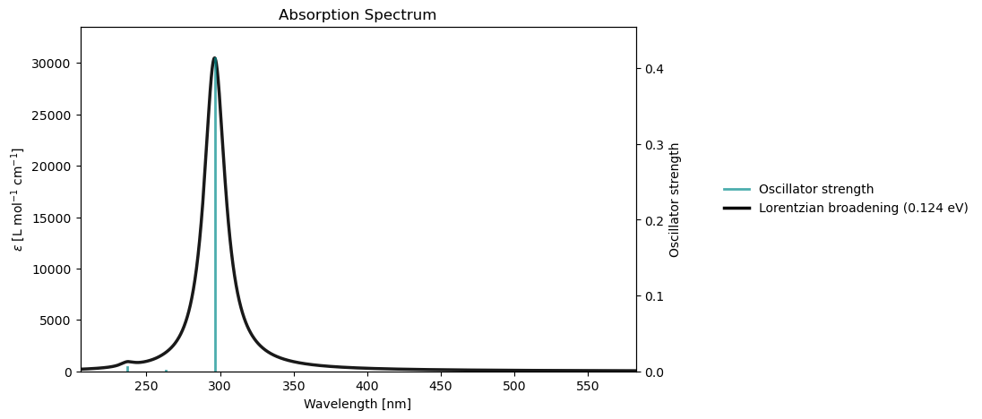
Text file
Please refer to the keyword list for a complete set of options. Note that natural transition orbitals NTO can be saved using the nto keyword. By specifying the absorption property, both UV/vis and ECD spectra will be calculated.
@jobs
task: response
@end

@method settings
xcfun: cam-b3lyp
basis: def2-svp
@end

@response
property: absorption
nstates: 10
nto: yes
@end

@molecule
charge: 0
multiplicity: 1
xyz:
...
@end
Complex polarization propagator approach
The linear absorption cross section can be determined directly from the imaginary part of the polarizability Norman et al. (2018)
where
and
The polarizability is complex and calculated with a damping term, ℏγ, associated with the inverse finite lifetime of the excited states. The default program setting for this parameter is 0.124 eV (or 0.004556 a.u.).
The resulting values for σ(ω) are presented in atomic units and can be converted to the SI unit of m2 by multiplying with a factor of a02.
The arbitrary frequency region is specified in the input file together with a requested frequency resolution.
Python script
import veloxchem as vlx
import numpy as np

molecule = vlx.Molecule.read_name("ethylene")
basis = vlx.MolecularBasis.read(molecule, "def2-svp")

scf_drv = vlx.ScfRestrictedDriver()
scf_drv.xcfun = "cam-b3lyp"
scf_results = scf_drv.compute(molecule, basis)

cpp_drv = vlx.ComplexResponse()
cpp_drv.frequencies = np.arange(0.2, 0.35, 0.0025)
cpp_drv.property = "absorption"

cpp_results = cpp_drv.compute(molecule, basis, scf_results)
Reading ethylene from PubChem...
Reference: S. Kim, J. Chen, T. Cheng, A. Gindulyte, J. He, S. He, Q. Li, B. A. Shoemaker, P. A. Thiessen, B. Yu, L. Zaslavsky, J. Zhang, E. E. Bolton, Nucleic Acids Res., 2025, 53, D1516-D1525.
Please double-check the compound since names may refer to more than one record.
Self Consistent Field Driver Setup
====================================
Wave Function Model : Spin-Restricted Kohn-Sham
Initial Guess Model : Superposition of Atomic Densities
Convergence Accelerator : Two Level Direct Inversion of Iterative Subspace
Max. Number of Iterations : 50
Max. Number of Error Vectors : 10
Convergence Threshold : 1.0e-06
ERI Screening Threshold : 1.0e-12
Linear Dependence Threshold : 1.0e-06
Exchange-Correlation Functional : CAM-B3LYP
Molecular Grid Level : 4
* Info * Using the CAM-B3LYP functional.
T. Yanai, D. P. Tew, and N. C. Handy., Chem. Phys. Lett. 393, 51 (2004)
* Info * Using the Libxc library (v7.0.0).
S. Lehtola, C. Steigemann, M. J.T. Oliveira, and M. A.L. Marques., SoftwareX 7, 1–5 (2018)
* Info * Using the following algorithm for XC numerical integration.
J. Kussmann, H. Laqua and C. Ochsenfeld, J. Chem. Theory Comput. 2021, 17, 1512-1521
* Info * Starting Reduced Basis SCF calculation...
* Info * ...done. SCF energy in reduced basis set: -77.938548735600 a.u. Time: 0.13 sec.
Iter. | Kohn-Sham Energy | Energy Change | Gradient Norm | Max. Gradient | Density Change
--------------------------------------------------------------------------------------------
1 -78.473052842120 0.0000000000 0.11746298 0.01322545 0.00000000
2 -78.473990049300 -0.0009372072 0.08911202 0.01182726 0.07840856
3 -78.475059198312 -0.0010691490 0.00183646 0.00037562 0.02599180
4 -78.475060232566 -0.0000010343 0.00026440 0.00007008 0.00211656
5 -78.475060252564 -0.0000000200 0.00004845 0.00000607 0.00024516
6 -78.475060252901 -0.0000000003 0.00000261 0.00000039 0.00002286
7 -78.475060252903 -0.0000000000 0.00000015 0.00000002 0.00000286
*** SCF converged in 7 iterations. Time: 1.27 sec.
Spin-Restricted Kohn-Sham:
--------------------------
Total Energy : -78.4750602529 a.u.
Electronic Energy : -111.8894772841 a.u.
Nuclear Repulsion Energy : 33.4144170312 a.u.
------------------------------------
Gradient Norm : 0.0000001531 a.u.
Ground State Information
------------------------
Charge of Molecule : 0.0
Multiplicity (2S+1) : 1
Magnetic Quantum Number (M_S) : 0.0
Complex Response Solver Setup
===============================
Number of Frequencies : 60
Max. Number of Iterations : 150
Convergence Threshold : 1.0e-04
ERI Screening Threshold : 1.0e-12
Exchange-Correlation Functional : CAM-B3LYP
Molecular Grid Level : 4
* Info * Using the CAM-B3LYP functional.
T. Yanai, D. P. Tew, and N. C. Handy., Chem. Phys. Lett. 393, 51 (2004)
* Info * Using the Libxc library (v7.0.0).
S. Lehtola, C. Steigemann, M. J.T. Oliveira, and M. A.L. Marques., SoftwareX 7, 1–5 (2018)
* Info * Using the following algorithm for XC numerical integration.
J. Kussmann, H. Laqua and C. Ochsenfeld, J. Chem. Theory Comput. 2021, 17, 1512-1521
* Info * 10 gerade trial vectors in reduced space
* Info * 11 ungerade trial vectors in reduced space
*** Iteration: 1 * Residuals (Max,Min): 4.60e-01 and 2.87e-01
* Info * 20 gerade trial vectors in reduced space
* Info * 21 ungerade trial vectors in reduced space
*** Iteration: 2 * Residuals (Max,Min): 3.38e-02 and 1.90e-02
* Info * 32 gerade trial vectors in reduced space
* Info * 34 ungerade trial vectors in reduced space
*** Iteration: 3 * Residuals (Max,Min): 5.32e-03 and 1.35e-03
* Info * 43 gerade trial vectors in reduced space
* Info * 46 ungerade trial vectors in reduced space
*** Iteration: 4 * Residuals (Max,Min): 3.43e-04 and 7.40e-05
* Info * 54 gerade trial vectors in reduced space
* Info * 59 ungerade trial vectors in reduced space
*** Iteration: 5 * Residuals (Max,Min): 9.85e-05 and 4.98e-06
*** Complex response converged in 5 iterations. Time: 37.43 sec
Linear Absorption Cross-Section
===============================
Reference: J. Kauczor and P. Norman, J. Chem. Theory Comput. 2014, 10, 2449-2455.
Frequency[a.u.] Frequency[eV] sigma(w)[a.u.]
-------------------------------------------------------
0.2000 5.44228 0.00735224
0.2025 5.51031 0.00777863
0.2050 5.57833 0.00823728
0.2075 5.64636 0.00873162
0.2100 5.71439 0.00926558
0.2125 5.78242 0.00984364
0.2150 5.85045 0.01047096
0.2175 5.91848 0.01115348
0.2200 5.98650 0.01189807
0.2225 6.05453 0.01271272
0.2250 6.12256 0.01360677
0.2275 6.19059 0.01459119
0.2300 6.25862 0.01567891
0.2325 6.32665 0.01688530
0.2350 6.39468 0.01822869
0.2375 6.46270 0.01973113
0.2400 6.53073 0.02141931
0.2425 6.59876 0.02332576
0.2450 6.66679 0.02549051
0.2475 6.73482 0.02796315
0.2500 6.80285 0.03080582
0.2525 6.87088 0.03409711
0.2550 6.93890 0.03793756
0.2575 7.00693 0.04245747
0.2600 7.07496 0.04782799
0.2625 7.14299 0.05427740
0.2650 7.21102 0.06211543
0.2675 7.27905 0.07177046
0.2700 7.34707 0.08384791
0.2725 7.41510 0.09922469
0.2750 7.48313 0.11920727
0.2775 7.55116 0.14580632
0.2800 7.61919 0.18223549
0.2825 7.68722 0.23386284
0.2850 7.75525 0.31013068
0.2875 7.82327 0.42867135
0.2900 7.89130 0.62465638
0.2925 7.95933 0.97254362
0.2950 8.02736 1.62889331
0.2975 8.09539 2.80563373
0.3000 8.16342 3.94422771
0.3025 8.23144 3.31066794
0.3050 8.29947 2.01022419
0.3075 8.36750 1.20036567
0.3100 8.43553 0.77035258
0.3125 8.50356 0.53419896
0.3150 8.57159 0.39860870
0.3175 8.63962 0.32143163
0.3200 8.70764 0.27553204
0.3225 8.77567 0.22737395
0.3250 8.84370 0.18028492
0.3275 8.91173 0.14672941
0.3300 8.97976 0.12357826
0.3325 9.04779 0.10687132
0.3350 9.11581 0.09431387
0.3375 9.18384 0.08460220
0.3400 9.25187 0.07694498
0.3425 9.31990 0.07083020
0.3450 9.38793 0.06590970
0.3475 9.45596 0.06193792
cpp_drv.plot(cpp_results)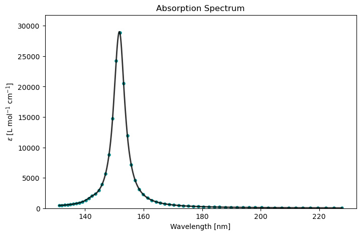
Text file
@jobs
task: response
@end

@method settings
xcfun: b3lyp
basis: def2-svp
@end

@response
property: absorption (cpp)
# frequency region (and resolution)
frequencies: 0.10-0.25 (0.0025)
damping: 0.0045563  # this is the default value
@end

@molecule
charge: 0
multiplicity: 1
xyz:
...
@end
Please refer to the keyword list for a complete set of options.
- Norman, P., Ruud, K., & Saue, T. (2018). Principles and practices of molecular properties. John Wiley & Sons, Ltd.