VeloxChem provides simulations of vibrational spectroscopies by evaluating molecular force constants and deriving normal modes whose frequencies and transition properties form the basis for IR and Raman spectra. Building on a converged ground‑state DFT reference, the program computes the molecular Hessian and transforms it to mass‑weighted internal coordinates to obtain physically meaningful vibrational modes, while subsequent response‑theory evaluations yield dipole‑derivative and polarizability‑derivative quantities that determine vibrational intensities. Together, these capabilities enable predictions of both harmonic vibrational frequencies and their associated infrared and Raman signatures.
The calculation of normal modes is performed with the aid of geomeTRIC.
Infrared
Infrared (IR) spectroscopy in VeloxChem is based on the calculation of harmonic vibrational frequencies and their dipole‑moment derivatives, which determine the intensity of each normal‑mode transition. Starting from a ground state DFT reference, the molecular Hessian is evaluated and transformed into mass‑weighted normal modes, whose frequencies and IR intensities together form the vibrational spectrum. See visualisation of normal modes and visualisation of spectra for interactive visualisation tools.
Python script
import veloxchem as vlx

molecule = vlx.Molecule.read_name("formaldehyde")
basis = vlx.MolecularBasis.read(molecule, "def2-svp")

scf_drv = vlx.ScfRestrictedDriver()
scf_drv.xcfun = "b3lyp"
results = scf_drv.compute(molecule, basis)

vib_drv = vlx.VibrationalAnalysis(scf_drv)
vib_drv.do_ir = True

vib_results = vib_drv.compute(molecule, basis)
Reading formaldehyde from PubChem...
Reference: S. Kim, J. Chen, T. Cheng, A. Gindulyte, J. He, S. He, Q. Li, B. A. Shoemaker, P. A. Thiessen, B. Yu, L. Zaslavsky, J. Zhang, E. E. Bolton, Nucleic Acids Res., 2025, 53, D1516-D1525.
Please double-check the compound since names may refer to more than one record.
Self Consistent Field Driver Setup
====================================
Wave Function Model : Spin-Restricted Kohn-Sham
Initial Guess Model : Superposition of Atomic Densities
Convergence Accelerator : Two Level Direct Inversion of Iterative Subspace
Max. Number of Iterations : 50
Max. Number of Error Vectors : 10
Convergence Threshold : 1.0e-06
ERI Screening Threshold : 1.0e-12
Linear Dependence Threshold : 1.0e-06
Exchange-Correlation Functional : B3LYP
Molecular Grid Level : 4
* Info * Using the B3LYP functional.
P. J. Stephens, F. J. Devlin, C. F. Chabalowski, and M. J. Frisch., J. Phys. Chem. 98, 11623 (1994)
* Info * Using the Libxc library (v7.0.0).
S. Lehtola, C. Steigemann, M. J.T. Oliveira, and M. A.L. Marques., SoftwareX 7, 1–5 (2018)
* Info * Using the following algorithm for XC numerical integration.
J. Kussmann, H. Laqua and C. Ochsenfeld, J. Chem. Theory Comput. 2021, 17, 1512-1521
* Info * Starting Reduced Basis SCF calculation...
* Info * ...done. SCF energy in reduced basis set: -113.714598841635 a.u. Time: 0.25 sec.
Iter. | Kohn-Sham Energy | Energy Change | Gradient Norm | Max. Gradient | Density Change
--------------------------------------------------------------------------------------------
1 -114.404173442505 0.0000000000 0.28750653 0.04292380 0.00000000
2 -114.404203719132 -0.0000302766 0.29053028 0.03775015 0.13977833
3 -114.412290874517 -0.0080871554 0.08909150 0.01050656 0.07989966
4 -114.413033900988 -0.0007430265 0.01505012 0.00173322 0.02720197
5 -114.413059518957 -0.0000256180 0.00084728 0.00009598 0.00599335
6 -114.413059607094 -0.0000000881 0.00008931 0.00001504 0.00030275
7 -114.413059608320 -0.0000000012 0.00002157 0.00000218 0.00003537
8 -114.413059608370 -0.0000000001 0.00000082 0.00000008 0.00000858
*** SCF converged in 8 iterations. Time: 1.19 sec.
Spin-Restricted Kohn-Sham:
--------------------------
Total Energy : -114.4130596084 a.u.
Electronic Energy : -145.6211440192 a.u.
Nuclear Repulsion Energy : 31.2080844109 a.u.
------------------------------------
Gradient Norm : 0.0000008166 a.u.
Ground State Information
------------------------
Charge of Molecule : 0.0
Multiplicity (2S+1) : 1
Magnetic Quantum Number (M_S) : 0.0
Vibrational Analysis Driver
=============================
The following will be computed:
- Vibrational frequencies and normal modes
- Force constants
- IR intensities
SCF Hessian Driver Setup
==========================
Hessian Type : Analytical
* Info * Computing analytical Hessian...
Reference: P. Deglmann, F. Furche, R. Ahlrichs, Chem. Phys. Lett. 2002, 362, 511-518.
* Info * Using the B3LYP functional.
P. J. Stephens, F. J. Devlin, C. F. Chabalowski, and M. J. Frisch., J. Phys. Chem. 98, 11623 (1994)
* Info * Using the Libxc library (v7.0.0).
S. Lehtola, C. Steigemann, M. J.T. Oliveira, and M. A.L. Marques., SoftwareX 7, 1–5 (2018)
* Info * Using the following algorithm for XC numerical integration.
J. Kussmann, H. Laqua and C. Ochsenfeld, J. Chem. Theory Comput. 2021, 17, 1512-1521
* Info * CPHF/CPKS integral derivatives computed in 14.03 sec.
* Info * CPHF/CPKS right-hand side computed in 2.14 sec.
Coupled-Perturbed Kohn-Sham Solver Setup
------------------------------------------
Solver Type : Iterative Subspace Algorithm
Max. Number of Iterations : 150
Convergence Threshold : 1.0e-04
Exchange-Correlation Functional : B3LYP
Molecular Grid Level : 4
* Info * 9 trial vectors in reduced space
*** Iteration: 1 * Residuals (Max,Min): 6.26e-01 and 1.06e-01
* Info * 18 trial vectors in reduced space
*** Iteration: 2 * Residuals (Max,Min): 5.85e-02 and 1.21e-02
* Info * 27 trial vectors in reduced space
*** Iteration: 3 * Residuals (Max,Min): 6.95e-03 and 8.81e-04
* Info * 35 trial vectors in reduced space
*** Iteration: 4 * Residuals (Max,Min): 5.29e-04 and 4.48e-05
* Info * 42 trial vectors in reduced space
*** Iteration: 5 * Residuals (Max,Min): 9.20e-05 and 1.09e-05
*** Coupled-Perturbed Kohn-Sham converged in 5 iterations. Time: 32.18 sec
* Info * First order derivative contributions to the Hessian computed in 0.00 sec.
* Info * Second order derivative contributions to the Hessian computed in 10.51 sec.
*** Time spent in Hessian calculation: 42.85 sec ***
Free Energy Analysis
======================
Note: Rotational symmetry is set to 1 regardless of true symmetry
No Imaginary Frequencies
Free energy contributions calculated at @ 298.15 K:
Zero-point vibrational energy: 17.1420 kcal/mol
H (Trans + Rot + Vib = Tot): 1.4812 + 0.8887 + 0.0311 = 2.4011 kcal/mol
S (Trans + Rot + Vib = Tot): 36.1564 + 17.4049 + 0.1228 = 53.6841 cal/mol/K
TS (Trans + Rot + Vib = Tot): 10.7800 + 5.1893 + 0.0366 = 16.0059 kcal/mol
Ground State Electronic Energy : E0 = -114.41305961 au ( -71795.2789 kcal/mol)
Free Energy Correction (Harmonic) : ZPVE + [H-TS]_T,R,V = 0.00563683 au ( 3.5372 kcal/mol)
Gibbs Free Energy (Harmonic) : E0 + ZPVE + [H-TS]_T,R,V = -114.40742278 au ( -71791.7417 kcal/mol)
Vibrational Analysis
======================
* Info * The 5 dominant normal modes are printed below.
Vibrational Mode 2
----------------------------------------------------
Harmonic frequency: 1213.97 cm**-1
Reduced mass: 1.3177 amu
Force constant: 1.1442 mdyne/A
IR intensity: 10.1124 km/mol
Normal mode:
X Y Z
1 C -0.0951 0.0309 0.1007
2 O 0.0516 -0.0167 -0.0546
3 H -0.0605 -0.6711 -0.1815
4 H 0.3744 0.5693 -0.1508
Vibrational Mode 3
----------------------------------------------------
Harmonic frequency: 1473.18 cm**-1
Reduced mass: 1.0833 amu
Force constant: 1.3853 mdyne/A
IR intensity: 5.1155 km/mol
Normal mode:
X Y Z
1 C -0.0030 -0.0085 -0.0002
2 O -0.0233 -0.0666 -0.0016
3 H -0.0302 0.6545 0.2611
4 H 0.4361 0.5032 -0.2325
Vibrational Mode 4
----------------------------------------------------
Harmonic frequency: 1745.33 cm**-1
Reduced mass: 8.7847 amu
Force constant: 15.7665 mdyne/A
IR intensity: 90.3622 km/mol
Normal mode:
X Y Z
1 C 0.2126 0.6062 0.0150
2 O -0.1538 -0.4386 -0.0108
3 H 0.2287 -0.2176 -0.2931
4 H -0.3190 -0.0399 0.2867
Vibrational Mode 5
----------------------------------------------------
Harmonic frequency: 3177.46 cm**-1
Reduced mass: 1.0415 amu
Force constant: 6.1955 mdyne/A
IR intensity: 42.5404 km/mol
Normal mode:
X Y Z
1 C 0.0183 0.0522 0.0013
2 O 0.0006 0.0017 0.0000
3 H -0.5271 -0.1897 0.4298
4 H 0.2999 -0.4581 -0.4457
Vibrational Mode 6
----------------------------------------------------
Harmonic frequency: 3296.85 cm**-1
Reduced mass: 1.1241 amu
Force constant: 7.1986 mdyne/A
IR intensity: 100.5187 km/mol
Normal mode:
X Y Z
1 C 0.0689 -0.0224 -0.0730
2 O -0.0002 0.0001 0.0002
3 H -0.5247 -0.1972 0.4249
4 H -0.2933 0.4627 0.4412
vib_drv.plot_ir(vib_results)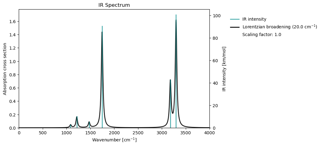
Text file
@jobs
task: vibrational
@end

@method settings
xcfun: b3lyp
basis: def2-svp
@end

@vibrational
do_ir: yes
@end

@molecule
charge: 0
multiplicity: 1
xyz:
...
@end
Raman
Raman spectroscopy in VeloxChem is based on evaluating harmonic vibrational frequencies together with the derivatives of the molecular polarizability tensor, which determine the Raman scattering strength of each normal mode. Using the Hessian, the normal modes are obtained in their mass‑weighted form and used to compute Raman intensities from the corresponding polarizability changes. This framework enables prediction of Raman‑active vibrational features and provides a complementary perspective to IR spectroscopy through polarizability‑based selection rules.
Python script
import veloxchem as vlx

molecule = vlx.Molecule.read_name("formaldehyde")
basis = vlx.MolecularBasis.read(molecule, "def2-svp")

scf_drv = vlx.ScfRestrictedDriver()
scf_drv.xcfun = "b3lyp"
results = scf_drv.compute(molecule, basis)

vib_drv = vlx.VibrationalAnalysis(scf_drv)
vib_drv.do_ir = False
vib_drv.do_raman = True

vib_results = vib_drv.compute(molecule, basis)
Reading formaldehyde from PubChem...
Reference: S. Kim, J. Chen, T. Cheng, A. Gindulyte, J. He, S. He, Q. Li, B. A. Shoemaker, P. A. Thiessen, B. Yu, L. Zaslavsky, J. Zhang, E. E. Bolton, Nucleic Acids Res., 2025, 53, D1516-D1525.
Please double-check the compound since names may refer to more than one record.
Self Consistent Field Driver Setup
====================================
Wave Function Model : Spin-Restricted Kohn-Sham
Initial Guess Model : Superposition of Atomic Densities
Convergence Accelerator : Two Level Direct Inversion of Iterative Subspace
Max. Number of Iterations : 50
Max. Number of Error Vectors : 10
Convergence Threshold : 1.0e-06
ERI Screening Threshold : 1.0e-12
Linear Dependence Threshold : 1.0e-06
Exchange-Correlation Functional : B3LYP
Molecular Grid Level : 4
* Info * Using the B3LYP functional.
P. J. Stephens, F. J. Devlin, C. F. Chabalowski, and M. J. Frisch., J. Phys. Chem. 98, 11623 (1994)
* Info * Using the Libxc library (v7.0.0).
S. Lehtola, C. Steigemann, M. J.T. Oliveira, and M. A.L. Marques., SoftwareX 7, 1–5 (2018)
* Info * Using the following algorithm for XC numerical integration.
J. Kussmann, H. Laqua and C. Ochsenfeld, J. Chem. Theory Comput. 2021, 17, 1512-1521
* Info * Starting Reduced Basis SCF calculation...
* Info * ...done. SCF energy in reduced basis set: -113.714598865636 a.u. Time: 2.05 sec.
Iter. | Kohn-Sham Energy | Energy Change | Gradient Norm | Max. Gradient | Density Change
--------------------------------------------------------------------------------------------
1 -114.404171961603 0.0000000000 0.28750917 0.04292440 0.00000000
2 -114.404201930517 -0.0000299689 0.29053862 0.03775112 0.13978046
3 -114.412289600724 -0.0080876702 0.08908948 0.01050627 0.07990102
4 -114.413032593551 -0.0007429928 0.01505011 0.00173321 0.02720170
5 -114.413058211515 -0.0000256180 0.00084728 0.00009598 0.00599340
6 -114.413058299652 -0.0000000881 0.00008930 0.00001504 0.00030276
7 -114.413058300878 -0.0000000012 0.00002157 0.00000218 0.00003536
8 -114.413058300929 -0.0000000001 0.00000082 0.00000008 0.00000859
*** SCF converged in 8 iterations. Time: 1.37 sec.
Spin-Restricted Kohn-Sham:
--------------------------
Total Energy : -114.4130583009 a.u.
Electronic Energy : -145.6211572168 a.u.
Nuclear Repulsion Energy : 31.2080989159 a.u.
------------------------------------
Gradient Norm : 0.0000008166 a.u.
Ground State Information
------------------------
Charge of Molecule : 0.0
Multiplicity (2S+1) : 1
Magnetic Quantum Number (M_S) : 0.0
Vibrational Analysis Driver
=============================
The following will be computed:
- Vibrational frequencies and normal modes
- Force constants
- Raman activity
SCF Hessian Driver Setup
==========================
Hessian Type : Analytical
* Info * Computing analytical Hessian...
Reference: P. Deglmann, F. Furche, R. Ahlrichs, Chem. Phys. Lett. 2002, 362, 511-518.
* Info * Using the B3LYP functional.
P. J. Stephens, F. J. Devlin, C. F. Chabalowski, and M. J. Frisch., J. Phys. Chem. 98, 11623 (1994)
* Info * Using the Libxc library (v7.0.0).
S. Lehtola, C. Steigemann, M. J.T. Oliveira, and M. A.L. Marques., SoftwareX 7, 1–5 (2018)
* Info * Using the following algorithm for XC numerical integration.
J. Kussmann, H. Laqua and C. Ochsenfeld, J. Chem. Theory Comput. 2021, 17, 1512-1521
* Info * CPHF/CPKS integral derivatives computed in 34.28 sec.
* Info * CPHF/CPKS right-hand side computed in 4.86 sec.
Coupled-Perturbed Kohn-Sham Solver Setup
------------------------------------------
Solver Type : Iterative Subspace Algorithm
Max. Number of Iterations : 150
Convergence Threshold : 1.0e-04
Exchange-Correlation Functional : B3LYP
Molecular Grid Level : 4
* Info * 9 trial vectors in reduced space
*** Iteration: 1 * Residuals (Max,Min): 4.61e-01 and 9.37e-02
* Info * 18 trial vectors in reduced space
*** Iteration: 2 * Residuals (Max,Min): 4.73e-02 and 1.13e-02
* Info * 27 trial vectors in reduced space
*** Iteration: 3 * Residuals (Max,Min): 5.56e-03 and 8.85e-04
* Info * 35 trial vectors in reduced space
*** Iteration: 4 * Residuals (Max,Min): 4.15e-04 and 6.26e-05
* Info * 41 trial vectors in reduced space
*** Iteration: 5 * Residuals (Max,Min): 6.58e-05 and 1.23e-05
*** Coupled-Perturbed Kohn-Sham converged in 5 iterations. Time: 86.00 sec
* Info * First order derivative contributions to the Hessian computed in 0.00 sec.
* Info * Second order derivative contributions to the Hessian computed in 10.10 sec.
*** Time spent in Hessian calculation: 96.11 sec ***
Linear Response Solver Setup
==============================
Number of Frequencies : 1
Max. Number of Iterations : 150
Convergence Threshold : 1.0e-04
ERI Screening Threshold : 1.0e-12
Exchange-Correlation Functional : B3LYP
Molecular Grid Level : 4
* Info * Using the B3LYP functional.
P. J. Stephens, F. J. Devlin, C. F. Chabalowski, and M. J. Frisch., J. Phys. Chem. 98, 11623 (1994)
* Info * Using the Libxc library (v7.0.0).
S. Lehtola, C. Steigemann, M. J.T. Oliveira, and M. A.L. Marques., SoftwareX 7, 1–5 (2018)
* Info * Using the following algorithm for XC numerical integration.
J. Kussmann, H. Laqua and C. Ochsenfeld, J. Chem. Theory Comput. 2021, 17, 1512-1521
* Info * 0 gerade trial vectors in reduced space
* Info * 3 ungerade trial vectors in reduced space
*** Iteration: 1 * Residuals (Max,Min): 1.08e+00 and 8.13e-01
* Info * 0 gerade trial vectors in reduced space
* Info * 6 ungerade trial vectors in reduced space
*** Iteration: 2 * Residuals (Max,Min): 1.17e-01 and 8.93e-02
* Info * 0 gerade trial vectors in reduced space
* Info * 9 ungerade trial vectors in reduced space
*** Iteration: 3 * Residuals (Max,Min): 2.98e-02 and 2.16e-02
* Info * 0 gerade trial vectors in reduced space
* Info * 12 ungerade trial vectors in reduced space
*** Iteration: 4 * Residuals (Max,Min): 4.65e-03 and 3.32e-03
* Info * 0 gerade trial vectors in reduced space
* Info * 15 ungerade trial vectors in reduced space
*** Iteration: 5 * Residuals (Max,Min): 3.69e-04 and 2.64e-04
* Info * 0 gerade trial vectors in reduced space
* Info * 18 ungerade trial vectors in reduced space
*** Iteration: 6 * Residuals (Max,Min): 6.16e-05 and 4.38e-05
*** Linear response converged in 6 iterations. Time: 7.46 sec
Polarizability (w=0.0000)
-------------------------
X Y Z
X 15.24140929 -2.04728188 -0.78514811
Y -2.04728188 13.87136169 3.88037784
Z -0.78514811 3.88037784 9.91138561
Polarizability Gradient Driver
================================
Polarizability gradient type : Real Analytical
* Info * Using the B3LYP functional.
P. J. Stephens, F. J. Devlin, C. F. Chabalowski, and M. J. Frisch., J. Phys. Chem. 98, 11623 (1994)
* Info * Using the Libxc library (v7.0.0).
S. Lehtola, C. Steigemann, M. J.T. Oliveira, and M. A.L. Marques., SoftwareX 7, 1–5 (2018)
* Info * Using the following algorithm for XC numerical integration.
J. Kussmann, H. Laqua and C. Ochsenfeld, J. Chem. Theory Comput. 2021, 17, 1512-1521
* Info * Building RHS for w = 0.000
* Info * 4.66 kB of memory used for subspace procedure on the master node
* Info * 4.91 GB of memory available for the solver on the master node
* Info * 394.54 kB of memory used for subspace procedure on the master node
* Info * 4.91 GB of memory available for the solver on the master node
* Info * ** Time spent on constructing the orbrsp RHS for 1 frequencies: 1.79 sec **
Coupled-Perturbed Kohn-Sham Solver Setup
------------------------------------------
Solver Type : Iterative Subspace Algorithm
Max. Number of Iterations : 150
Convergence Threshold : 1.0e-04
Number of frequencies : 1
Vector components : xyz
* Info * 6 trial vectors in reduced space
*** Iteration: 1 * Residuals (Max,Min): 1.27e-01 and 7.33e-02
* Info * 12 trial vectors in reduced space
*** Iteration: 2 * Residuals (Max,Min): 1.87e-02 and 8.67e-03
* Info * 18 trial vectors in reduced space
*** Iteration: 3 * Residuals (Max,Min): 2.65e-03 and 1.04e-03
* Info * 24 trial vectors in reduced space
*** Iteration: 4 * Residuals (Max,Min): 2.20e-04 and 1.07e-04
* Info * 30 trial vectors in reduced space
*** Iteration: 5 * Residuals (Max,Min): 1.44e-05 and 9.71e-06
*** Coupled-Perturbed Kohn-Sham converged in 5 iterations. Time: 9.48 sec
* Info * Using the B3LYP functional.
P. J. Stephens, F. J. Devlin, C. F. Chabalowski, and M. J. Frisch., J. Phys. Chem. 98, 11623 (1994)
* Info * Using the Libxc library (v7.0.0).
S. Lehtola, C. Steigemann, M. J.T. Oliveira, and M. A.L. Marques., SoftwareX 7, 1–5 (2018)
* Info * Using the following algorithm for XC numerical integration.
J. Kussmann, H. Laqua and C. Ochsenfeld, J. Chem. Theory Comput. 2021, 17, 1512-1521
* Info * Building omega for w = 0.000
* Info * 69.62 kB of memory used for subspace procedure on the master node
* Info * 4.85 GB of memory available for the solver on the master node
** Time spent on constructing omega multipliers for 1 frequencies: 2.98 sec **
* Info * Building gradient for frequency = 0.000
* Info * 396.00 bytes of memory used for subspace procedure on the master node
* Info * 4.84 GB of memory available for the solver on the master node
* Info * ** Time spent on constructing the analytical gradient for 1 frequencies: 27.78 sec **
*** Time spent in polarizability gradient driver: 40.32 sec ***
Free Energy Analysis
======================
Note: Rotational symmetry is set to 1 regardless of true symmetry
No Imaginary Frequencies
Free energy contributions calculated at @ 298.15 K:
Zero-point vibrational energy: 17.1420 kcal/mol
H (Trans + Rot + Vib = Tot): 1.4812 + 0.8887 + 0.0311 = 2.4011 kcal/mol
S (Trans + Rot + Vib = Tot): 36.1564 + 17.4049 + 0.1228 = 53.6841 cal/mol/K
TS (Trans + Rot + Vib = Tot): 10.7800 + 5.1893 + 0.0366 = 16.0059 kcal/mol
Ground State Electronic Energy : E0 = -114.41305830 au ( -71795.2780 kcal/mol)
Free Energy Correction (Harmonic) : ZPVE + [H-TS]_T,R,V = 0.00563685 au ( 3.5372 kcal/mol)
Gibbs Free Energy (Harmonic) : E0 + ZPVE + [H-TS]_T,R,V = -114.40742146 au ( -71791.7409 kcal/mol)
Vibrational Analysis
======================
* Info * The 5 lowest normal modes are printed below.
Vibrational Mode 1
----------------------------------------------------
Harmonic frequency: 1084.21 cm**-1
Reduced mass: 1.3445 amu
Force constant: 0.9312 mdyne/A
Raman activity: static 0.6321 A**4/amu
Normal mode:
X Y Z
1 C -0.0094 -0.0901 0.1427
2 O 0.0022 0.0208 -0.0329
3 H 0.0386 0.3712 -0.5879
4 H 0.0386 0.3712 -0.5879
Vibrational Mode 2
----------------------------------------------------
Harmonic frequency: 1213.97 cm**-1
Reduced mass: 1.3177 amu
Force constant: 1.1442 mdyne/A
Raman activity: static 7.6961 A**4/amu
Normal mode:
X Y Z
1 C -0.1107 -0.0715 -0.0524
2 O 0.0600 0.0388 0.0284
3 H 0.5921 -0.3286 -0.1686
4 H -0.2266 0.5647 0.3417
Vibrational Mode 3
----------------------------------------------------
Harmonic frequency: 1473.19 cm**-1
Reduced mass: 1.0833 amu
Force constant: 1.3853 mdyne/A
Raman activity: static 11.8140 A**4/amu
Normal mode:
X Y Z
1 C 0.0056 -0.0061 -0.0035
2 O 0.0439 -0.0479 -0.0274
3 H -0.6536 0.2415 0.1095
4 H -0.1106 0.5923 0.3667
Vibrational Mode 4
----------------------------------------------------
Harmonic frequency: 1745.34 cm**-1
Reduced mass: 8.7848 amu
Force constant: 15.7667 mdyne/A
Raman activity: static 5.3842 A**4/amu
Normal mode:
X Y Z
1 C 0.4001 -0.4366 -0.2494
2 O -0.2895 0.3158 0.1804
3 H -0.4038 -0.1133 -0.0980
4 H 0.2339 0.2987 0.2040
Vibrational Mode 5
----------------------------------------------------
Harmonic frequency: 3177.46 cm**-1
Reduced mass: 1.0415 amu
Force constant: 6.1955 mdyne/A
Raman activity: static 168.1788 A**4/amu
Normal mode:
X Y Z
1 C -0.0345 0.0376 0.0215
2 O -0.0011 0.0012 0.0007
3 H -0.2677 -0.5443 -0.3613
4 H 0.6953 0.0778 0.0948
vib_drv.plot_raman(vib_results)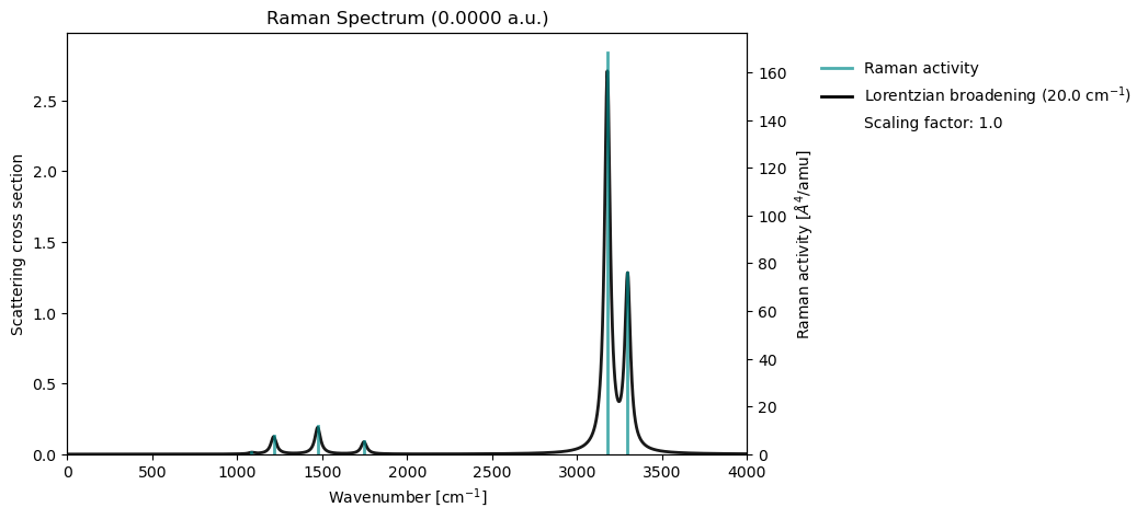
Text file
@jobs
task: vibrational
@end

@method settings
xcfun: b3lyp
basis: def2-svp
@end

@vibrational
do_raman: yes
@end

@molecule
charge: 0
multiplicity: 1
xyz:
...
@end
Resonance Raman
In resonance Raman spectroscopy, the vibrational intensities are selectively amplified when the excitation frequency is tuned close to an allowed electronic transition; in practice, we are often concerned with the spectrum at the transition energy of the first excited state (S1).
VeloxChem implements resonance Raman spectroscopy based on geometric derivatives of the complex polarizability. For further details on this approach, see Saidi & Norman (2014).
import veloxchem as vlx

molecule = vlx.Molecule.read_name("formaldehyde")
basis = vlx.MolecularBasis.read(molecule, "def2-svp")

scf_drv = vlx.ScfRestrictedDriver()
scf_drv.xcfun = "cam-b3lyp"
scf_results = scf_drv.compute(molecule, basis)

rsp_drv = vlx.LinearResponseEigenSolver()
rsp_drv.nstates = 5
rsp_results = rsp_drv.compute(molecule, basis, scf_results)
Reading formaldehyde from PubChem...
Reference: S. Kim, J. Chen, T. Cheng, A. Gindulyte, J. He, S. He, Q. Li, B. A. Shoemaker, P. A. Thiessen, B. Yu, L. Zaslavsky, J. Zhang, E. E. Bolton, Nucleic Acids Res., 2025, 53, D1516-D1525.
Please double-check the compound since names may refer to more than one record.
Self Consistent Field Driver Setup
====================================
Wave Function Model : Spin-Restricted Kohn-Sham
Initial Guess Model : Superposition of Atomic Densities
Convergence Accelerator : Two Level Direct Inversion of Iterative Subspace
Max. Number of Iterations : 50
Max. Number of Error Vectors : 10
Convergence Threshold : 1.0e-06
ERI Screening Threshold : 1.0e-12
Linear Dependence Threshold : 1.0e-06
Exchange-Correlation Functional : CAM-B3LYP
Molecular Grid Level : 4
* Info * Using the CAM-B3LYP functional.
T. Yanai, D. P. Tew, and N. C. Handy., Chem. Phys. Lett. 393, 51 (2004)
* Info * Using the Libxc library (v7.0.0).
S. Lehtola, C. Steigemann, M. J.T. Oliveira, and M. A.L. Marques., SoftwareX 7, 1–5 (2018)
* Info * Using the following algorithm for XC numerical integration.
J. Kussmann, H. Laqua and C. Ochsenfeld, J. Chem. Theory Comput. 2021, 17, 1512-1521
* Info * Starting Reduced Basis SCF calculation...
* Info * ...done. SCF energy in reduced basis set: -113.714598826273 a.u. Time: 0.25 sec.
Iter. | Kohn-Sham Energy | Energy Change | Gradient Norm | Max. Gradient | Density Change
--------------------------------------------------------------------------------------------
1 -114.356949058491 0.0000000000 0.21813714 0.03113800 0.00000000
2 -114.359717359465 -0.0027683010 0.15343024 0.01999022 0.09679622
3 -114.361633284620 -0.0019159252 0.06919554 0.00835328 0.04714156
4 -114.362068411155 -0.0004351265 0.00973873 0.00114344 0.01642425
5 -114.362078181737 -0.0000097706 0.00098393 0.00011404 0.00405253
6 -114.362078348377 -0.0000001666 0.00008560 0.00001054 0.00075069
7 -114.362078351730 -0.0000000034 0.00003675 0.00000339 0.00014049
8 -114.362078351900 -0.0000000002 0.00000322 0.00000032 0.00002121
9 -114.362078351902 -0.0000000000 0.00000039 0.00000004 0.00000201
*** SCF converged in 9 iterations. Time: 4.08 sec.
Spin-Restricted Kohn-Sham:
--------------------------
Total Energy : -114.3620783519 a.u.
Electronic Energy : -145.5701691585 a.u.
Nuclear Repulsion Energy : 31.2080908066 a.u.
------------------------------------
Gradient Norm : 0.0000003881 a.u.
Ground State Information
------------------------
Charge of Molecule : 0.0
Multiplicity (2S+1) : 1
Magnetic Quantum Number (M_S) : 0.0
Linear Response EigenSolver Setup
===================================
Number of States : 5
Max. Number of Iterations : 150
Convergence Threshold : 1.0e-04
ERI Screening Threshold : 1.0e-12
Exchange-Correlation Functional : CAM-B3LYP
Molecular Grid Level : 4
* Info * Using the CAM-B3LYP functional.
T. Yanai, D. P. Tew, and N. C. Handy., Chem. Phys. Lett. 393, 51 (2004)
* Info * Using the Libxc library (v7.0.0).
S. Lehtola, C. Steigemann, M. J.T. Oliveira, and M. A.L. Marques., SoftwareX 7, 1–5 (2018)
* Info * Using the following algorithm for XC numerical integration.
J. Kussmann, H. Laqua and C. Ochsenfeld, J. Chem. Theory Comput. 2021, 17, 1512-1521
* Info * 5 gerade trial vectors in reduced space
* Info * 5 ungerade trial vectors in reduced space
*** Iteration: 1 * Residuals (Max,Min): 7.56e-01 and 1.02e-01
* Info * 10 gerade trial vectors in reduced space
* Info * 10 ungerade trial vectors in reduced space
*** Iteration: 2 * Residuals (Max,Min): 8.57e-02 and 1.43e-02
* Info * 15 gerade trial vectors in reduced space
* Info * 15 ungerade trial vectors in reduced space
*** Iteration: 3 * Residuals (Max,Min): 1.76e-02 and 2.94e-03
* Info * 20 gerade trial vectors in reduced space
* Info * 20 ungerade trial vectors in reduced space
*** Iteration: 4 * Residuals (Max,Min): 1.58e-01 and 2.47e-04
* Info * 25 gerade trial vectors in reduced space
* Info * 25 ungerade trial vectors in reduced space
*** Iteration: 5 * Residuals (Max,Min): 1.96e-02 and 2.27e-05
* Info * 29 gerade trial vectors in reduced space
* Info * 29 ungerade trial vectors in reduced space
*** Iteration: 6 * Residuals (Max,Min): 2.08e-03 and 1.72e-05
* Info * 31 gerade trial vectors in reduced space
* Info * 31 ungerade trial vectors in reduced space
*** Iteration: 7 * Residuals (Max,Min): 1.02e-03 and 1.67e-05
* Info * 32 gerade trial vectors in reduced space
* Info * 32 ungerade trial vectors in reduced space
*** Iteration: 8 * Residuals (Max,Min): 1.01e-04 and 1.54e-05
* Info * 33 gerade trial vectors in reduced space
* Info * 33 ungerade trial vectors in reduced space
*** Iteration: 9 * Residuals (Max,Min): 6.34e-05 and 5.57e-06
*** Linear response converged in 9 iterations. Time: 21.03 sec
Electric Transition Dipole Moments (dipole length, a.u.)
--------------------------------------------------------
X Y Z
Excited State S1: -0.000001 -0.000001 -0.000000
Excited State S2: 0.320799 0.399607 0.571635
Excited State S3: 0.066006 -0.047516 -0.003826
Excited State S4: -0.151728 -0.230607 0.246354
Excited State S5: 0.000001 0.000002 -0.000001
Electric Transition Dipole Moments (dipole velocity, a.u.)
----------------------------------------------------------
X Y Z
Excited State S1: 0.000001 -0.000002 -0.000001
Excited State S2: 0.295003 0.367473 0.525667
Excited State S3: 0.125209 -0.090135 -0.007258
Excited State S4: -0.110281 -0.167613 0.179058
Excited State S5: 0.000001 0.000003 -0.000000
Magnetic Transition Dipole Moments (a.u.)
-----------------------------------------
X Y Z
Excited State S1: 0.249941 0.379882 -0.405828
Excited State S2: 0.389771 -0.727566 0.289876
Excited State S3: 0.315186 0.396723 0.510660
Excited State S4: -0.029966 -0.146802 -0.155873
Excited State S5: -0.142935 -0.217238 0.232082
One-Photon Absorption
---------------------
Excited State S1: 0.14191110 a.u. 3.86160 eV Osc.Str. 0.0000
Excited State S2: 0.32011855 a.u. 8.71087 eV Osc.Str. 0.1258
Excited State S3: 0.32742622 a.u. 8.90972 eV Osc.Str. 0.0014
Excited State S4: 0.35400328 a.u. 9.63292 eV Osc.Str. 0.0323
Excited State S5: 0.38638565 a.u. 10.51409 eV Osc.Str. 0.0000
Electronic Circular Dichroism
-----------------------------
Excited State S1: Rot.Str. -0.000000 a.u. -0.0001 [10**(-40) cgs]
Excited State S2: Rot.Str. 0.000001 a.u. 0.0006 [10**(-40) cgs]
Excited State S3: Rot.Str. -0.000001 a.u. -0.0003 [10**(-40) cgs]
Excited State S4: Rot.Str. 0.000000 a.u. 0.0001 [10**(-40) cgs]
Excited State S5: Rot.Str. -0.000001 a.u. -0.0004 [10**(-40) cgs]
Character of excitations:
Excited state 1
---------------
HOMO -> LUMO 0.9993
Excited state 2
---------------
HOMO -> LUMO+1 0.9959
Excited state 3
---------------
HOMO-2 -> LUMO -0.9976
Excited state 4
---------------
HOMO-1 -> LUMO 0.8263
HOMO -> LUMO+2 0.5451
Excited state 5
---------------
HOMO-3 -> LUMO 0.9975
molecule.show()print(f"S1 excitation energy: {rsp_results["eigenvalues"][0]:10.6f} (a.u.)")S1 excitation energy: 0.141911 (a.u.)
Python script
import veloxchem as vlx
import numpy as np

molecule = vlx.Molecule.read_name("formaldehyde")
basis = vlx.MolecularBasis.read(molecule, "def2-svp")

scf_drv = vlx.ScfRestrictedDriver()
scf_drv.xcfun = "b3lyp"
scf_results = scf_drv.compute(molecule, basis)

vib_drv = vlx.VibrationalAnalysis(scf_drv)
vib_drv.do_ir = False
vib_drv.do_raman = False
vib_drv.do_resonance_raman = True

vib_drv.frequencies = [0.141911]

vib_results = vib_drv.compute(molecule, basis)
Reading formaldehyde from PubChem...
Reference: S. Kim, J. Chen, T. Cheng, A. Gindulyte, J. He, S. He, Q. Li, B. A. Shoemaker, P. A. Thiessen, B. Yu, L. Zaslavsky, J. Zhang, E. E. Bolton, Nucleic Acids Res., 2025, 53, D1516-D1525.
Please double-check the compound since names may refer to more than one record.
Self Consistent Field Driver Setup
====================================
Wave Function Model : Spin-Restricted Kohn-Sham
Initial Guess Model : Superposition of Atomic Densities
Convergence Accelerator : Two Level Direct Inversion of Iterative Subspace
Max. Number of Iterations : 50
Max. Number of Error Vectors : 10
Convergence Threshold : 1.0e-06
ERI Screening Threshold : 1.0e-12
Linear Dependence Threshold : 1.0e-06
Exchange-Correlation Functional : B3LYP
Molecular Grid Level : 4
* Info * Using the B3LYP functional.
P. J. Stephens, F. J. Devlin, C. F. Chabalowski, and M. J. Frisch., J. Phys. Chem. 98, 11623 (1994)
* Info * Using the Libxc library (v7.0.0).
S. Lehtola, C. Steigemann, M. J.T. Oliveira, and M. A.L. Marques., SoftwareX 7, 1–5 (2018)
* Info * Using the following algorithm for XC numerical integration.
J. Kussmann, H. Laqua and C. Ochsenfeld, J. Chem. Theory Comput. 2021, 17, 1512-1521
* Info * Starting Reduced Basis SCF calculation...
* Info * ...done. SCF energy in reduced basis set: -113.714598844189 a.u. Time: 0.22 sec.
Iter. | Kohn-Sham Energy | Energy Change | Gradient Norm | Max. Gradient | Density Change
--------------------------------------------------------------------------------------------
1 -114.404173111804 0.0000000000 0.28750775 0.04292404 0.00000000
2 -114.404203305848 -0.0000301940 0.29053303 0.03775048 0.13977911
3 -114.412290633842 -0.0080873280 0.08909080 0.01050645 0.07990002
4 -114.413033648770 -0.0007430149 0.01505006 0.00173321 0.02720183
5 -114.413059266568 -0.0000256178 0.00084727 0.00009598 0.00599332
6 -114.413059354702 -0.0000000881 0.00008931 0.00001504 0.00030275
7 -114.413059355928 -0.0000000012 0.00002157 0.00000218 0.00003537
8 -114.413059355978 -0.0000000001 0.00000082 0.00000008 0.00000858
*** SCF converged in 8 iterations. Time: 5.40 sec.
Spin-Restricted Kohn-Sham:
--------------------------
Total Energy : -114.4130593560 a.u.
Electronic Energy : -145.6211522277 a.u.
Nuclear Repulsion Energy : 31.2080928717 a.u.
------------------------------------
Gradient Norm : 0.0000008166 a.u.
Ground State Information
------------------------
Charge of Molecule : 0.0
Multiplicity (2S+1) : 1
Magnetic Quantum Number (M_S) : 0.0
Vibrational Analysis Driver
=============================
The following will be computed:
- Vibrational frequencies and normal modes
- Force constants
- Resonance Raman (1 frequencies)
SCF Hessian Driver Setup
==========================
Hessian Type : Analytical
* Info * Computing analytical Hessian...
Reference: P. Deglmann, F. Furche, R. Ahlrichs, Chem. Phys. Lett. 2002, 362, 511-518.
* Info * Using the B3LYP functional.
P. J. Stephens, F. J. Devlin, C. F. Chabalowski, and M. J. Frisch., J. Phys. Chem. 98, 11623 (1994)
* Info * Using the Libxc library (v7.0.0).
S. Lehtola, C. Steigemann, M. J.T. Oliveira, and M. A.L. Marques., SoftwareX 7, 1–5 (2018)
* Info * Using the following algorithm for XC numerical integration.
J. Kussmann, H. Laqua and C. Ochsenfeld, J. Chem. Theory Comput. 2021, 17, 1512-1521
* Info * CPHF/CPKS integral derivatives computed in 29.87 sec.
* Info * CPHF/CPKS right-hand side computed in 5.28 sec.
Coupled-Perturbed Kohn-Sham Solver Setup
------------------------------------------
Solver Type : Iterative Subspace Algorithm
Max. Number of Iterations : 150
Convergence Threshold : 1.0e-04
Exchange-Correlation Functional : B3LYP
Molecular Grid Level : 4
* Info * 9 trial vectors in reduced space
*** Iteration: 1 * Residuals (Max,Min): 5.69e-01 and 1.07e-01
* Info * 18 trial vectors in reduced space
*** Iteration: 2 * Residuals (Max,Min): 5.49e-02 and 1.32e-02
* Info * 27 trial vectors in reduced space
*** Iteration: 3 * Residuals (Max,Min): 6.52e-03 and 9.54e-04
* Info * 35 trial vectors in reduced space
*** Iteration: 4 * Residuals (Max,Min): 4.96e-04 and 6.00e-05
* Info * 42 trial vectors in reduced space
*** Iteration: 5 * Residuals (Max,Min): 8.76e-05 and 8.98e-06
*** Coupled-Perturbed Kohn-Sham converged in 5 iterations. Time: 64.09 sec
* Info * First order derivative contributions to the Hessian computed in 0.00 sec.
* Info * Second order derivative contributions to the Hessian computed in 11.30 sec.
*** Time spent in Hessian calculation: 75.41 sec ***
Complex Response Solver Setup
===============================
Number of Frequencies : 1
Max. Number of Iterations : 150
Convergence Threshold : 1.0e-04
ERI Screening Threshold : 1.0e-12
Exchange-Correlation Functional : B3LYP
Molecular Grid Level : 4
* Info * Using the B3LYP functional.
P. J. Stephens, F. J. Devlin, C. F. Chabalowski, and M. J. Frisch., J. Phys. Chem. 98, 11623 (1994)
* Info * Using the Libxc library (v7.0.0).
S. Lehtola, C. Steigemann, M. J.T. Oliveira, and M. A.L. Marques., SoftwareX 7, 1–5 (2018)
* Info * Using the following algorithm for XC numerical integration.
J. Kussmann, H. Laqua and C. Ochsenfeld, J. Chem. Theory Comput. 2021, 17, 1512-1521
* Info * 6 gerade trial vectors in reduced space
* Info * 6 ungerade trial vectors in reduced space
*** Iteration: 1 * Residuals (Max,Min): 9.97e-01 and 3.02e-01
* Info * 11 gerade trial vectors in reduced space
* Info * 12 ungerade trial vectors in reduced space
*** Iteration: 2 * Residuals (Max,Min): 9.08e-02 and 3.27e-02
* Info * 16 gerade trial vectors in reduced space
* Info * 17 ungerade trial vectors in reduced space
*** Iteration: 3 * Residuals (Max,Min): 1.34e-02 and 3.71e-03
* Info * 21 gerade trial vectors in reduced space
* Info * 21 ungerade trial vectors in reduced space
*** Iteration: 4 * Residuals (Max,Min): 1.63e-03 and 3.36e-04
* Info * 24 gerade trial vectors in reduced space
* Info * 26 ungerade trial vectors in reduced space
*** Iteration: 5 * Residuals (Max,Min): 1.74e-04 and 2.89e-05
* Info * 27 gerade trial vectors in reduced space
* Info * 29 ungerade trial vectors in reduced space
*** Iteration: 6 * Residuals (Max,Min): 2.89e-05 and 5.85e-06
*** Complex response converged in 6 iterations. Time: 8.67 sec
Linear Absorption Cross-Section
===============================
Reference: J. Kauczor and P. Norman, J. Chem. Theory Comput. 2014, 10, 2449-2455.
Frequency[a.u.] Frequency[eV] sigma(w)[a.u.]
-------------------------------------------------------
0.1419 3.86160 0.00109414
Polarizability Gradient Driver
================================
Polarizability gradient type : Complex Analytical
Damping value : 0.0046 a.u.
* Info * Using the B3LYP functional.
P. J. Stephens, F. J. Devlin, C. F. Chabalowski, and M. J. Frisch., J. Phys. Chem. 98, 11623 (1994)
* Info * Using the Libxc library (v7.0.0).
S. Lehtola, C. Steigemann, M. J.T. Oliveira, and M. A.L. Marques., SoftwareX 7, 1–5 (2018)
* Info * Using the following algorithm for XC numerical integration.
J. Kussmann, H. Laqua and C. Ochsenfeld, J. Chem. Theory Comput. 2021, 17, 1512-1521
* Info * Building RHS for w = 0.142
* Info * 14.42 kB of memory used for subspace procedure on the master node
* Info * 4.78 GB of memory available for the solver on the master node
* Info * 1.21 MB of memory used for subspace procedure on the master node
* Info * 4.78 GB of memory available for the solver on the master node
* Info * ** Time spent on constructing the orbrsp RHS for 1 frequencies: 19.30 sec **
Coupled-Perturbed Kohn-Sham Solver Setup
------------------------------------------
Solver Type : Iterative Subspace Algorithm
Max. Number of Iterations : 150
Convergence Threshold : 1.0e-04
Number of frequencies : 1
Vector components : xyz
* Info * 12 trial vectors in reduced space
*** Iteration: 1 * Residuals (Max,Min): 1.53e-01 and 4.42e-02
* Info * 23 trial vectors in reduced space
*** Iteration: 2 * Residuals (Max,Min): 1.60e-02 and 5.48e-03
* Info * 31 trial vectors in reduced space
*** Iteration: 3 * Residuals (Max,Min): 2.48e-03 and 4.45e-04
* Info * 41 trial vectors in reduced space
*** Iteration: 4 * Residuals (Max,Min): 1.31e-04 and 2.12e-05
* Info * 49 trial vectors in reduced space
*** Iteration: 5 * Residuals (Max,Min): 8.95e-05 and 4.21e-06
*** Coupled-Perturbed Kohn-Sham converged in 5 iterations. Time: 39.96 sec
* Info * Using the B3LYP functional.
P. J. Stephens, F. J. Devlin, C. F. Chabalowski, and M. J. Frisch., J. Phys. Chem. 98, 11623 (1994)
* Info * Using the Libxc library (v7.0.0).
S. Lehtola, C. Steigemann, M. J.T. Oliveira, and M. A.L. Marques., SoftwareX 7, 1–5 (2018)
* Info * Using the following algorithm for XC numerical integration.
J. Kussmann, H. Laqua and C. Ochsenfeld, J. Chem. Theory Comput. 2021, 17, 1512-1521
* Info * Building omega for w = 0.142
* Info * 139.16 kB of memory used for subspace procedure on the master node
* Info * 4.75 GB of memory available for the solver on the master node
** Time spent on constructing omega multipliers for 1 frequencies: 1.22 sec **
* Info * Building gradient for frequency = 0.142
* Info * 392.00 bytes of memory used for subspace procedure on the master node
* Info * 4.74 GB of memory available for the solver on the master node
* Info * ** Time spent on constructing the analytical gradient for 1 frequencies: 94.60 sec **
*** Time spent in polarizability gradient driver: 135.91 sec ***
Free Energy Analysis
======================
Note: Rotational symmetry is set to 1 regardless of true symmetry
No Imaginary Frequencies
Free energy contributions calculated at @ 298.15 K:
Zero-point vibrational energy: 17.1420 kcal/mol
H (Trans + Rot + Vib = Tot): 1.4812 + 0.8887 + 0.0311 = 2.4011 kcal/mol
S (Trans + Rot + Vib = Tot): 36.1564 + 17.4049 + 0.1228 = 53.6841 cal/mol/K
TS (Trans + Rot + Vib = Tot): 10.7800 + 5.1893 + 0.0366 = 16.0059 kcal/mol
Ground State Electronic Energy : E0 = -114.41305936 au ( -71795.2787 kcal/mol)
Free Energy Correction (Harmonic) : ZPVE + [H-TS]_T,R,V = 0.00563683 au ( 3.5372 kcal/mol)
Gibbs Free Energy (Harmonic) : E0 + ZPVE + [H-TS]_T,R,V = -114.40742252 au ( -71791.7415 kcal/mol)
Vibrational Analysis
======================
* Info * The 5 lowest normal modes are printed below.
Vibrational Mode 1
----------------------------------------------------
Harmonic frequency: 1084.20 cm**-1
Reduced mass: 1.3445 amu
Force constant: 0.9312 mdyne/A
Normal mode:
X Y Z
1 C -0.1316 0.0471 -0.0950
2 O 0.0304 -0.0109 0.0219
3 H 0.5422 -0.1941 0.3916
4 H 0.5422 -0.1941 0.3916
Vibrational Mode 2
----------------------------------------------------
Harmonic frequency: 1213.97 cm**-1
Reduced mass: 1.3177 amu
Force constant: 1.1442 mdyne/A
Normal mode:
X Y Z
1 C -0.0885 -0.0625 0.0916
2 O 0.0480 0.0339 -0.0496
3 H 0.1907 -0.4577 -0.4910
4 H 0.1015 0.6641 0.1887
Vibrational Mode 3
----------------------------------------------------
Harmonic frequency: 1473.19 cm**-1
Reduced mass: 1.0833 amu
Force constant: 1.3853 mdyne/A
Normal mode:
X Y Z
1 C 0.0006 -0.0077 -0.0047
2 O 0.0048 -0.0602 -0.0365
3 H -0.2587 0.3702 0.5417
4 H 0.1754 0.6769 0.0927
Vibrational Mode 4
----------------------------------------------------
Harmonic frequency: 1745.33 cm**-1
Reduced mass: 8.7848 amu
Force constant: 15.7666 mdyne/A
Normal mode:
X Y Z
1 C 0.0436 -0.5483 -0.3322
2 O -0.0316 0.3967 0.2403
3 H -0.2641 -0.0636 0.3342
4 H 0.2456 0.2965 -0.1931
Vibrational Mode 5
----------------------------------------------------
Harmonic frequency: 3177.46 cm**-1
Reduced mass: 1.0415 amu
Force constant: 6.1955 mdyne/A
Normal mode:
X Y Z
1 C -0.0038 0.0472 0.0286
2 O -0.0001 0.0015 0.0009
3 H -0.3616 -0.5648 0.2207
4 H 0.4082 -0.0211 -0.5757
Resonance Raman
=================
Vibrational Mode 1
----------------------------------------------------
Frequency (a.u.) Raman activity (A**4/amu)
----------------------------------------------------
0.141911 0.6463
Vibrational Mode 2
----------------------------------------------------
Frequency (a.u.) Raman activity (A**4/amu)
----------------------------------------------------
0.141911 9.9214
Vibrational Mode 3
----------------------------------------------------
Frequency (a.u.) Raman activity (A**4/amu)
----------------------------------------------------
0.141911 14.3502
Vibrational Mode 4
----------------------------------------------------
Frequency (a.u.) Raman activity (A**4/amu)
----------------------------------------------------
0.141911 10.0218
Vibrational Mode 5
----------------------------------------------------
Frequency (a.u.) Raman activity (A**4/amu)
----------------------------------------------------
0.141911 260.9682
Vibrational Mode 6
----------------------------------------------------
Frequency (a.u.) Raman activity (A**4/amu)
----------------------------------------------------
0.141911 114.6912
vib_drv.plot_raman(vib_results)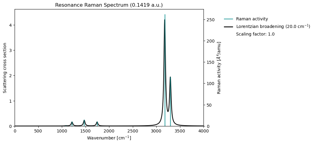
Text file
@jobs
task: vibrational
@end

@method settings
xcfun: b3lyp
basis: def2-svp
@end

@vibrational
do_resonance_raman: yes
frequencies: 0.05-0.10 (0.05)
@end

@molecule
charge: 0
multiplicity: 1
xyz:
...
@end- Saidi, W. A., & Norman, P. (2014). Probing single-walled carbon nanotube defect chemistry using resonance Raman spectroscopy. Carbon, 67, 17–26. 10.1016/j.carbon.2013.09.045