The calculation of molecular polarizabilities in VeloxChem is based on linear‑response theory, where the induced dipole moment is evaluated as a function of an external electric field to obtain the polarizability tensor. Starting from the ground state DFT reference, the frequency‑dependent response equations are solved to provide both static and dynamic polarizabilities, which serve as the foundation for describing optical properties such as refractive indices and light‑scattering behavior.
The linear electric-dipole polarizabilty is determined from the linear response function
where μ^α is the electric-dipole operator along Cartesian axis α and ω is the optical angular frequency. For randomly oriented samples, the relevant quantity is the isotropic polarizability
The atomic unit of polarizability is
At optical frequencies well separated from transition frequencies in the system, the polarizability is real, whereas in near-resonance or resonance regions of the spectrum, it becomes complex. For further theoretical details, see Norman et al. (2018).
Nonresonant region
In the nonresonant region, where the driving field lies far from any electronic transition, the molecular polarizability varies smoothly with frequency, and the response is dominated by elastic Rayleigh scattering arising from the real part of the polarizability tensor, while the imaginary component remains vanishingly small due to the absence of absorption.
Python script
import veloxchem as vlx

molecule = vlx.Molecule.read_name("methane")
basis = vlx.MolecularBasis.read(molecule, "def2-svpd")

scf_drv = vlx.ScfRestrictedDriver()
scf_drv.xcfun = "b3lyp"
scf_results = scf_drv.compute(molecule, basis)

lr_drv = vlx.LinearResponseSolver()

lr_drv.property = "polarizability"
lr_drv.frequencies = [0.0, 0.0656]  # static field is default

lr_results = lr_drv.compute(molecule, basis, scf_results)
Reading methane from PubChem...
Reference: S. Kim, J. Chen, T. Cheng, A. Gindulyte, J. He, S. He, Q. Li, B. A. Shoemaker, P. A. Thiessen, B. Yu, L. Zaslavsky, J. Zhang, E. E. Bolton, Nucleic Acids Res., 2025, 53, D1516-D1525.
Please double-check the compound since names may refer to more than one record.
Self Consistent Field Driver Setup
====================================
Wave Function Model : Spin-Restricted Kohn-Sham
Initial Guess Model : Superposition of Atomic Densities
Convergence Accelerator : Two Level Direct Inversion of Iterative Subspace
Max. Number of Iterations : 50
Max. Number of Error Vectors : 10
Convergence Threshold : 1.0e-06
ERI Screening Threshold : 1.0e-12
Linear Dependence Threshold : 1.0e-06
Exchange-Correlation Functional : B3LYP
Molecular Grid Level : 4
* Info * Using the B3LYP functional.
P. J. Stephens, F. J. Devlin, C. F. Chabalowski, and M. J. Frisch., J. Phys. Chem. 98, 11623 (1994)
* Info * Using the Libxc library (v7.0.0).
S. Lehtola, C. Steigemann, M. J.T. Oliveira, and M. A.L. Marques., SoftwareX 7, 1–5 (2018)
* Info * Using the following algorithm for XC numerical integration.
J. Kussmann, H. Laqua and C. Ochsenfeld, J. Chem. Theory Comput. 2021, 17, 1512-1521
* Info * Starting Reduced Basis SCF calculation...
* Info * ...done. SCF energy in reduced basis set: -40.144465271372 a.u. Time: 0.06 sec.
Iter. | Kohn-Sham Energy | Energy Change | Gradient Norm | Max. Gradient | Density Change
--------------------------------------------------------------------------------------------
1 -40.488723681112 0.0000000000 0.11236481 0.01304585 0.00000000
2 -40.488584431215 0.0001392499 0.11963957 0.01310453 0.06672170
3 -40.490477528752 -0.0018930975 0.00136171 0.00017702 0.03892728
4 -40.490477771469 -0.0000002427 0.00001510 0.00000133 0.00091517
5 -40.490477771509 -0.0000000000 0.00000332 0.00000044 0.00002433
6 -40.490477771511 -0.0000000000 0.00000004 0.00000000 0.00000275
*** SCF converged in 6 iterations. Time: 1.69 sec.
Spin-Restricted Kohn-Sham:
--------------------------
Total Energy : -40.4904777715 a.u.
Electronic Energy : -53.6909150039 a.u.
Nuclear Repulsion Energy : 13.2004372324 a.u.
------------------------------------
Gradient Norm : 0.0000000424 a.u.
Ground State Information
------------------------
Charge of Molecule : 0.0
Multiplicity (2S+1) : 1
Magnetic Quantum Number (M_S) : 0.0
Linear Response Solver Setup
==============================
Number of Frequencies : 2
Max. Number of Iterations : 150
Convergence Threshold : 1.0e-04
ERI Screening Threshold : 1.0e-12
Exchange-Correlation Functional : B3LYP
Molecular Grid Level : 4
* Info * Using the B3LYP functional.
P. J. Stephens, F. J. Devlin, C. F. Chabalowski, and M. J. Frisch., J. Phys. Chem. 98, 11623 (1994)
* Info * Using the Libxc library (v7.0.0).
S. Lehtola, C. Steigemann, M. J.T. Oliveira, and M. A.L. Marques., SoftwareX 7, 1–5 (2018)
* Info * Using the following algorithm for XC numerical integration.
J. Kussmann, H. Laqua and C. Ochsenfeld, J. Chem. Theory Comput. 2021, 17, 1512-1521
* Info * 3 gerade trial vectors in reduced space
* Info * 6 ungerade trial vectors in reduced space
*** Iteration: 1 * Residuals (Max,Min): 2.42e-01 and 2.38e-01
* Info * 6 gerade trial vectors in reduced space
* Info * 12 ungerade trial vectors in reduced space
*** Iteration: 2 * Residuals (Max,Min): 2.67e-02 and 2.64e-02
* Info * 9 gerade trial vectors in reduced space
* Info * 17 ungerade trial vectors in reduced space
*** Iteration: 3 * Residuals (Max,Min): 9.44e-04 and 9.33e-04
* Info * 12 gerade trial vectors in reduced space
* Info * 21 ungerade trial vectors in reduced space
*** Iteration: 4 * Residuals (Max,Min): 5.76e-05 and 4.93e-05
*** Linear response converged in 4 iterations. Time: 3.56 sec
Polarizability (w=0.0000)
-------------------------
X Y Z
X 17.22943399 0.00000919 0.00000408
Y 0.00000919 17.22943879 0.00000864
Z 0.00000408 0.00000864 17.22944035
Polarizability (w=0.0656)
-------------------------
X Y Z
X 17.50292715 0.00000955 0.00000422
Y 0.00000955 17.50293218 0.00000897
Z 0.00000422 0.00000897 17.50293382
print("Frequency      Polarizability (isotropic)")

for freq in lr_drv.frequencies:
    alpha_iso = 0
    for comp in "xyz":
        alpha_iso += lr_results["response_functions"][(comp, comp, freq)]
    alpha_iso = -alpha_iso / 3

    print(f"{freq:.4f} a.u. {alpha_iso:10.4f} a.u.")
Frequency Polarizability (isotropic)
0.0000 a.u. 17.2294 a.u.
0.0656 a.u. 17.5029 a.u.
Text file
@jobs
task: response
@end

@method settings
basis: aug-cc-pvdz
@end

@response
property: polarizability
frequencies: 0-0.25 (0.05)
@end

@molecule
charge: 0
multiplicity: 1
xyz:
...
@end
Resonant region
In the resonant region, the molecular polarizability exhibits strong frequency dependence as the probing field approaches an electronic transition, leading to large dispersive features in the real part and the emergence of an imaginary component directly associated with absorption and radiative damping processes.
Python script
import numpy as np
import veloxchem as vlx

molecule = vlx.Molecule.read_name("methane")
basis = vlx.MolecularBasis.read(molecule, "def2-svpd")

scf_drv = vlx.ScfRestrictedDriver()
scf_drv.xcfun = "b3lyp"
scf_results = scf_drv.compute(molecule, basis)

crs = vlx.ComplexResponse()

# to be implemented (together with a plot function)
# crs.property = "polarizability"

crs.a_operator = "electric dipole"
crs.b_operator = "electric dipole"

crs.a_components = ["x", "y", "z"]
crs.b_components = ["x", "y", "z"]

crs.frequencies = np.arange(0.3, 0.42, 0.0025)

crs_results = crs.compute(molecule, basis, scf_results)
Reading methane from PubChem...
Reference: S. Kim, J. Chen, T. Cheng, A. Gindulyte, J. He, S. He, Q. Li, B. A. Shoemaker, P. A. Thiessen, B. Yu, L. Zaslavsky, J. Zhang, E. E. Bolton, Nucleic Acids Res., 2025, 53, D1516-D1525.
Please double-check the compound since names may refer to more than one record.
Self Consistent Field Driver Setup
====================================
Wave Function Model : Spin-Restricted Kohn-Sham
Initial Guess Model : Superposition of Atomic Densities
Convergence Accelerator : Two Level Direct Inversion of Iterative Subspace
Max. Number of Iterations : 50
Max. Number of Error Vectors : 10
Convergence Threshold : 1.0e-06
ERI Screening Threshold : 1.0e-12
Linear Dependence Threshold : 1.0e-06
Exchange-Correlation Functional : B3LYP
Molecular Grid Level : 4
* Info * Using the B3LYP functional.
P. J. Stephens, F. J. Devlin, C. F. Chabalowski, and M. J. Frisch., J. Phys. Chem. 98, 11623 (1994)
* Info * Using the Libxc library (v7.0.0).
S. Lehtola, C. Steigemann, M. J.T. Oliveira, and M. A.L. Marques., SoftwareX 7, 1–5 (2018)
* Info * Using the following algorithm for XC numerical integration.
J. Kussmann, H. Laqua and C. Ochsenfeld, J. Chem. Theory Comput. 2021, 17, 1512-1521
* Info * Starting Reduced Basis SCF calculation...
* Info * ...done. SCF energy in reduced basis set: -40.144465251276 a.u. Time: 0.05 sec.
Iter. | Kohn-Sham Energy | Energy Change | Gradient Norm | Max. Gradient | Density Change
--------------------------------------------------------------------------------------------
1 -40.488724151329 0.0000000000 0.11236552 0.01304593 0.00000000
2 -40.488584905925 0.0001392454 0.11964009 0.01308449 0.06672203
3 -40.490478020113 -0.0018931142 0.00136170 0.00017675 0.03892746
4 -40.490478262826 -0.0000002427 0.00001510 0.00000130 0.00091515
5 -40.490478262867 -0.0000000000 0.00000332 0.00000044 0.00002433
6 -40.490478262868 -0.0000000000 0.00000004 0.00000000 0.00000275
*** SCF converged in 6 iterations. Time: 1.23 sec.
Spin-Restricted Kohn-Sham:
--------------------------
Total Energy : -40.4904782629 a.u.
Electronic Energy : -53.6909127033 a.u.
Nuclear Repulsion Energy : 13.2004344404 a.u.
------------------------------------
Gradient Norm : 0.0000000426 a.u.
Ground State Information
------------------------
Charge of Molecule : 0.0
Multiplicity (2S+1) : 1
Magnetic Quantum Number (M_S) : 0.0
Complex Response Solver Setup
===============================
Number of Frequencies : 48
Max. Number of Iterations : 150
Convergence Threshold : 1.0e-04
ERI Screening Threshold : 1.0e-12
Exchange-Correlation Functional : B3LYP
Molecular Grid Level : 4
* Info * Using the B3LYP functional.
P. J. Stephens, F. J. Devlin, C. F. Chabalowski, and M. J. Frisch., J. Phys. Chem. 98, 11623 (1994)
* Info * Using the Libxc library (v7.0.0).
S. Lehtola, C. Steigemann, M. J.T. Oliveira, and M. A.L. Marques., SoftwareX 7, 1–5 (2018)
* Info * Using the following algorithm for XC numerical integration.
J. Kussmann, H. Laqua and C. Ochsenfeld, J. Chem. Theory Comput. 2021, 17, 1512-1521
* Info * 12 gerade trial vectors in reduced space
* Info * 14 ungerade trial vectors in reduced space
*** Iteration: 1 * Residuals (Max,Min): 1.45e-01 and 7.64e-02
* Info * 27 gerade trial vectors in reduced space
* Info * 29 ungerade trial vectors in reduced space
*** Iteration: 2 * Residuals (Max,Min): 1.27e-02 and 4.24e-03
* Info * 41 gerade trial vectors in reduced space
* Info * 43 ungerade trial vectors in reduced space
*** Iteration: 3 * Residuals (Max,Min): 4.31e-04 and 1.61e-04
* Info * 54 gerade trial vectors in reduced space
* Info * 59 ungerade trial vectors in reduced space
*** Iteration: 4 * Residuals (Max,Min): 2.51e-05 and 4.70e-06
*** Complex response converged in 4 iterations. Time: 25.87 sec
import matplotlib.pyplot as plt
import numpy as np
from scipy.interpolate import CubicSpline

alpha_iso = []
for freq in crs.frequencies:
    diag = 0
    for comp in "xyz":
        key = (comp, comp, freq)
        diag += crs_results["response_functions"][key]
    alpha_iso.append(-diag/3)

alpha_iso = np.array(alpha_iso)

alpha_real = alpha_iso.real
alpha_imag = alpha_iso.imag

freqs = np.array(crs.frequencies)

# Cubic spline interpolation
cs_real = CubicSpline(freqs, alpha_real)
cs_imag = CubicSpline(freqs, alpha_imag)

# Dense grid for smooth curves
f_dense = np.linspace(freqs.min(), freqs.max(), 400)

# Create figure and axis
fig, ax = plt.subplots()

# --- Smooth cubic-spline curves ---
ax.plot(f_dense, cs_real(f_dense), "-", linewidth=1.4, label="real part")
ax.plot(f_dense, cs_imag(f_dense), "-", linewidth=1.4, label="imag part")

ax.set_xlim(0.3, 0.42)
plt.title("Polarizability")
ax.set_xlabel("Frequency (a.u.)")
ax.set_ylabel(r"$\overline{\alpha}(\omega)$ (a.u.)")
ax.grid(True)
ax.legend()

plt.show()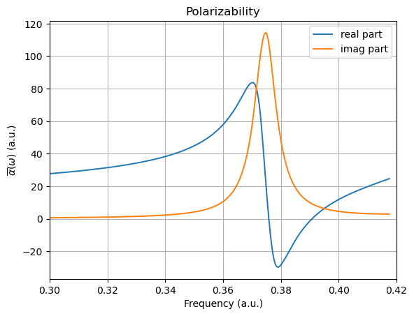
- Norman, P., Ruud, K., & Saue, T. (2018). Principles and practices of molecular properties. John Wiley & Sons, Ltd.