VeloxChem enables simulations of molecular optical activity by providing access to rotatory strengths, specific rotations, circular dichroism (ECD) spectra, and optical rotatory dispersion (ORD) through density‑functional theory response methods. These chiroptical properties can be obtained either from an eigenvalue‑based TDDFT treatment of excited states or through the complex polarization propagator (CPP) approach, which delivers frequency‑dependent spectra directly comparable to experiment. For systems composed of weakly interacting chromophores, VeloxChem also implements an exciton coupling model to compute ECD spectra from the interactions between local excitations. For further theoretical details, see Norman et al. (2018).
In this section, (S)-methyloxirane is used to showcase the calculations of rotatory strengths via TDDFT, extinction coefficients via CPP, and specific rotations and ORD via CPP. Finally, the exciton coupling model (ECM) is illustrated using a helical stack of ethylene molecules.
import veloxchem as vlx
molecule = vlx.Molecule.read_xyz_string("""10

O             -1.009866880244         1.299407071912         1.951947754409
C              0.031038818173         2.001294498224         1.244371321259
C              0.339506903623         0.795807201271         2.029917688849
C              0.600316751832        -0.544462572436         1.394186918859
H             -0.026285836651         1.930258644799         0.154459855148
H              0.271804379347         2.990968281608         1.641505800108
H              0.794935917667         0.948100885444         3.014899839267
H              0.113110324011        -0.610670447580         0.412641743927
H              1.681576973773        -0.701096452623         1.264343536564
H              0.213803265264        -1.354101659046         2.029564064183""")
molecule.show()Rotatory strengths
The strength of an ECD band is given by the anisotropy of the decadic molar extinction coefficient
where NA is Avogadro’s constant, f is the Cauchy distribution, and Rn0 is the rotatory strength defined as
In VeloxChem, the rotatory strength is evaluated in the velocity gauge as given in the second expression, and it is thereby gauge-origin independent.
Python script
import veloxchem as vlx

molecule = vlx.Molecule.read_xyz_string("""10

O             -1.009866880244         1.299407071912         1.951947754409
C              0.031038818173         2.001294498224         1.244371321259
C              0.339506903623         0.795807201271         2.029917688849
C              0.600316751832        -0.544462572436         1.394186918859
H             -0.026285836651         1.930258644799         0.154459855148
H              0.271804379347         2.990968281608         1.641505800108
H              0.794935917667         0.948100885444         3.014899839267
H              0.113110324011        -0.610670447580         0.412641743927
H              1.681576973773        -0.701096452623         1.264343536564
H              0.213803265264        -1.354101659046         2.029564064183""")


basis = vlx.MolecularBasis.read(molecule, "aug-cc-pvdz")

scf_drv = vlx.ScfRestrictedDriver()
scf_drv.xcfun = "b3lyp"
scf_results = scf_drv.compute(molecule, basis)

rsp_drv = vlx.LinearResponseEigenSolver()
rsp_drv.nstates = 8
rsp_results = rsp_drv.compute(molecule, basis, scf_results)
                                            Self Consistent Field Driver Setup
                                           ====================================

                   Wave Function Model             : Spin-Restricted Kohn-Sham
                   Initial Guess Model             : Superposition of Atomic Densities
                   Convergence Accelerator         : Two Level Direct Inversion of Iterative Subspace
                   Max. Number of Iterations       : 50
                   Max. Number of Error Vectors    : 10
                   Convergence Threshold           : 1.0e-06
                   ERI Screening Threshold         : 1.0e-12
                   Linear Dependence Threshold     : 1.0e-06
                   Exchange-Correlation Functional : B3LYP
                   Molecular Grid Level            : 4

* Info * Using the B3LYP functional.

         P. J. Stephens, F. J. Devlin, C. F. Chabalowski, and M. J. Frisch.,  J. Phys. Chem. 98, 11623 (1994)

* Info * Using the Libxc library (v7.0.0).

         S. Lehtola, C. Steigemann, M. J.T. Oliveira, and M. A.L. Marques.,  SoftwareX 7, 1–5 (2018)

* Info * Using the following algorithm for XC numerical integration.

         J. Kussmann, H. Laqua and C. Ochsenfeld, J. Chem. Theory Comput. 2021, 17, 1512-1521

* Info * Starting Reduced Basis SCF calculation...
* Info * ...done. SCF energy in reduced basis set: -191.823960423869 a.u. Time: 0.20 sec.


               Iter. |    Kohn-Sham Energy | Energy Change | Gradient Norm | Max. Gradient | Density Change
               --------------------------------------------------------------------------------------------
                  1      -193.118458872835    0.0000000000      0.37554496      0.01584480      0.00000000
                  2      -193.123363772891   -0.0049049001      0.31279732      0.01116367      0.35290190
                  3      -193.133247393175   -0.0098836203      0.09723785      0.00344749      0.19548399
                  4      -193.134034399260   -0.0007870061      0.02578568      0.00095366      0.03577760
                  5      -193.134110134095   -0.0000757348      0.00220004      0.00009796      0.01460491
                  6      -193.134110453179   -0.0000003191      0.00150842      0.00005205      0.00186854
                  7      -193.134110721512   -0.0000002683      0.00019811      0.00000712      0.00088667
                  8      -193.134110726432   -0.0000000049      0.00004901      0.00000196      0.00011428
                  9      -193.134110726716   -0.0000000003      0.00001349      0.00000071      0.00003271
                 10      -193.134110726739   -0.0000000000      0.00000258      0.00000012      0.00000770
                 11      -193.134110726739   -0.0000000000      0.00000033      0.00000002      0.00000182

               *** SCF converged in 11 iterations. Time: 3.61 sec.

               Spin-Restricted Kohn-Sham:
               --------------------------
               Total Energy                       :     -193.1341107267 a.u.
               Electronic Energy                  :     -317.2229127196 a.u.
               Nuclear Repulsion Energy           :      124.0888019929 a.u.
               ------------------------------------
               Gradient Norm                      :        0.0000003314 a.u.


               Ground State Information
               ------------------------
               Charge of Molecule            :  0.0
               Multiplicity (2S+1)           :  1
               Magnetic Quantum Number (M_S) :  0.0


                                            Linear Response EigenSolver Setup
                                           ===================================

                               Number of States                : 8
                               Max. Number of Iterations       : 150
                               Convergence Threshold           : 1.0e-04
                               ERI Screening Threshold         : 1.0e-12
                               Exchange-Correlation Functional : B3LYP
                               Molecular Grid Level            : 4

* Info * Using the B3LYP functional.

         P. J. Stephens, F. J. Devlin, C. F. Chabalowski, and M. J. Frisch.,  J. Phys. Chem. 98, 11623 (1994)

* Info * Using the Libxc library (v7.0.0).

         S. Lehtola, C. Steigemann, M. J.T. Oliveira, and M. A.L. Marques.,  SoftwareX 7, 1–5 (2018)

* Info * Using the following algorithm for XC numerical integration.

         J. Kussmann, H. Laqua and C. Ochsenfeld, J. Chem. Theory Comput. 2021, 17, 1512-1521

* Info * 24 gerade trial vectors in reduced space
* Info * 24 ungerade trial vectors in reduced space

               *** Iteration:   1 * Residuals (Max,Min): 8.68e-02 and 4.35e-02

* Info * 32 gerade trial vectors in reduced space
* Info * 32 ungerade trial vectors in reduced space

               *** Iteration:   2 * Residuals (Max,Min): 2.48e-02 and 1.46e-02

* Info * 40 gerade trial vectors in reduced space
* Info * 40 ungerade trial vectors in reduced space

               *** Iteration:   3 * Residuals (Max,Min): 6.90e-03 and 3.94e-03

* Info * 48 gerade trial vectors in reduced space
* Info * 48 ungerade trial vectors in reduced space

               *** Iteration:   4 * Residuals (Max,Min): 2.30e-03 and 6.17e-04

* Info * 56 gerade trial vectors in reduced space
* Info * 56 ungerade trial vectors in reduced space

               *** Iteration:   5 * Residuals (Max,Min): 1.04e-03 and 8.11e-05

* Info * 62 gerade trial vectors in reduced space
* Info * 62 ungerade trial vectors in reduced space

               *** Iteration:   6 * Residuals (Max,Min): 1.84e-04 and 1.70e-05

* Info * 63 gerade trial vectors in reduced space
* Info * 63 ungerade trial vectors in reduced space

               *** Iteration:   7 * Residuals (Max,Min): 7.44e-05 and 1.64e-05

               *** Linear response converged in 7 iterations. Time: 17.06 sec


               Electric Transition Dipole Moments (dipole length, a.u.)
               --------------------------------------------------------
                                                X            Y            Z
               Excited State    S1:     -0.217293    -0.026544    -0.147996
               Excited State    S2:     -0.238252    -0.064194    -0.027731
               Excited State    S3:      0.079786     0.347230     0.188537
               Excited State    S4:      0.131910    -0.002991     0.142636
               Excited State    S5:     -0.008054     0.159260    -0.105377
               Excited State    S6:      0.103602     0.015077    -0.168438
               Excited State    S7:     -0.070045     0.109074    -0.145301
               Excited State    S8:      0.154707    -0.120654    -0.157189

               Electric Transition Dipole Moments (dipole velocity, a.u.)
               ----------------------------------------------------------
                                                X            Y            Z
               Excited State    S1:     -0.215452    -0.026328    -0.144560
               Excited State    S2:     -0.230424    -0.061787    -0.025908
               Excited State    S3:      0.078891     0.347358     0.191358
               Excited State    S4:      0.133749    -0.000038     0.145455
               Excited State    S5:     -0.011574     0.160112    -0.106695
               Excited State    S6:      0.096852     0.020448    -0.167401
               Excited State    S7:     -0.066892     0.108397    -0.145870
               Excited State    S8:      0.156212    -0.117558    -0.154998

               Magnetic Transition Dipole Moments (a.u.)
               -----------------------------------------
                                                X            Y            Z
               Excited State    S1:     -0.161196    -0.003560    -0.049271
               Excited State    S2:      0.091828     0.025875     0.012814
               Excited State    S3:     -0.122014     0.056924    -0.072189
               Excited State    S4:      0.057418     0.259708    -0.130036
               Excited State    S5:      0.047962    -0.017591     0.152137
               Excited State    S6:     -0.167335     0.141036    -0.041169
               Excited State    S7:     -0.110507     0.114029     0.020632
               Excited State    S8:      0.054433     0.008957     0.061604

               One-Photon Absorption
               ---------------------
               Excited State    S1:      0.23958167 a.u.      6.51935 eV    Osc.Str.    0.0112
               Excited State    S2:      0.25585587 a.u.      6.96219 eV    Osc.Str.    0.0105
               Excited State    S3:      0.25721471 a.u.      6.99917 eV    Osc.Str.    0.0279
               Excited State    S4:      0.26004798 a.u.      7.07627 eV    Osc.Str.    0.0065
               Excited State    S5:      0.27134198 a.u.      7.38359 eV    Osc.Str.    0.0066
               Excited State    S6:      0.28549215 a.u.      7.76864 eV    Osc.Str.    0.0075
               Excited State    S7:      0.28872189 a.u.      7.85652 eV    Osc.Str.    0.0073
               Excited State    S8:      0.28941043 a.u.      7.87526 eV    Osc.Str.    0.0122

               Electronic Circular Dichroism
               -----------------------------
               Excited State    S1:     Rot.Str.      0.041946 a.u.    19.7754 [10**(-40) cgs]
               Excited State    S2:     Rot.Str.     -0.023090 a.u.   -10.8857 [10**(-40) cgs]
               Excited State    S3:     Rot.Str.     -0.003667 a.u.    -1.7286 [10**(-40) cgs]
               Excited State    S4:     Rot.Str.     -0.011245 a.u.    -5.3012 [10**(-40) cgs]
               Excited State    S5:     Rot.Str.     -0.019604 a.u.    -9.2422 [10**(-40) cgs]
               Excited State    S6:     Rot.Str.     -0.006431 a.u.    -3.0319 [10**(-40) cgs]
               Excited State    S7:     Rot.Str.      0.016743 a.u.     7.8933 [10**(-40) cgs]
               Excited State    S8:     Rot.Str.     -0.002098 a.u.    -0.9892 [10**(-40) cgs]

               Character of excitations:

               Excited state 1
               ---------------
               HOMO     -> LUMO         0.9834

               Excited state 2
               ---------------
               HOMO     -> LUMO+2      -0.9605

               Excited state 3
               ---------------
               HOMO     -> LUMO+1      -0.9583

               Excited state 4
               ---------------
               HOMO     -> LUMO+3      -0.8888
               HOMO     -> LUMO+5       0.2620
               HOMO     -> LUMO+2       0.2285

               Excited state 5
               ---------------
               HOMO-1   -> LUMO         0.9897

               Excited state 6
               ---------------
               HOMO     -> LUMO+4      -0.9664

               Excited state 7
               ---------------
               HOMO-1   -> LUMO+2       0.9202
               HOMO-1   -> LUMO+1      -0.2451
               HOMO     -> LUMO+5       0.2203

               Excited state 8
               ---------------
               HOMO     -> LUMO+5      -0.7954
               HOMO     -> LUMO+6      -0.3420
               HOMO-1   -> LUMO+1      -0.3270
               HOMO     -> LUMO+3      -0.2966
rsp_drv.plot_ecd(rsp_results)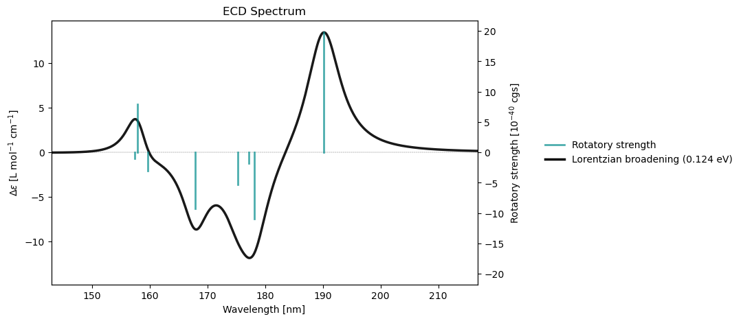
Text file
@jobs
task: response
@end

@method settings
basis: def2-svpd
xcfun: b3lyp
@end

@response
property: ecd
nstates: 10
nto: yes
@end

@molecule
charge: 0
multiplicity: 1
xyz:
...
@end
Extinction coefficient
The anisotropy of the decadic molar extinction coefficient can be determined directly from the complex polarization propagator evaluated for mixed electric- and magnetic-dipole operators Jiemchooroj & Norman (2007)
where the molecular response property, β(ω), is defined as
and
The mixed electric–magnetic dipole tensor, G, is evaluated in the velocity gauge as given in the second expression. Furthermore, it is complex and calculated with a damping term, ℏγ, associated with the inverse finite lifetime of the excited states. The default program setting for this parameter is 0.124 eV (or 0.004556 a.u.).
The resulting values for Δϵ(ω) are converted from atomic units to units of L mol−1 cm−1 by multiplying with a factor of 10a02.
Python script
import numpy as np
import veloxchem as vlx

molecule = vlx.Molecule.read_xyz_string("""10

O             -1.009866880244         1.299407071912         1.951947754409
C              0.031038818173         2.001294498224         1.244371321259
C              0.339506903623         0.795807201271         2.029917688849
C              0.600316751832        -0.544462572436         1.394186918859
H             -0.026285836651         1.930258644799         0.154459855148
H              0.271804379347         2.990968281608         1.641505800108
H              0.794935917667         0.948100885444         3.014899839267
H              0.113110324011        -0.610670447580         0.412641743927
H              1.681576973773        -0.701096452623         1.264343536564
H              0.213803265264        -1.354101659046         2.029564064183""")

basis = vlx.MolecularBasis.read(molecule, "aug-cc-pvdz")

scf_drv = vlx.ScfRestrictedDriver()
scf_drv.xcfun = "b3lyp"
scf_results = scf_drv.compute(molecule, basis)

cpp_drv = vlx.ComplexResponse()
cpp_drv.frequencies = np.arange(0.207, 0.325, 0.0025)
cpp_drv.property = "ecd"

cpp_results = cpp_drv.compute(molecule, basis, scf_results)
                                            Self Consistent Field Driver Setup
                                           ====================================

                   Wave Function Model             : Spin-Restricted Kohn-Sham
                   Initial Guess Model             : Superposition of Atomic Densities
                   Convergence Accelerator         : Two Level Direct Inversion of Iterative Subspace
                   Max. Number of Iterations       : 50
                   Max. Number of Error Vectors    : 10
                   Convergence Threshold           : 1.0e-06
                   ERI Screening Threshold         : 1.0e-12
                   Linear Dependence Threshold     : 1.0e-06
                   Exchange-Correlation Functional : B3LYP
                   Molecular Grid Level            : 4

* Info * Using the B3LYP functional.

         P. J. Stephens, F. J. Devlin, C. F. Chabalowski, and M. J. Frisch.,  J. Phys. Chem. 98, 11623 (1994)

* Info * Using the Libxc library (v7.0.0).

         S. Lehtola, C. Steigemann, M. J.T. Oliveira, and M. A.L. Marques.,  SoftwareX 7, 1–5 (2018)

* Info * Using the following algorithm for XC numerical integration.

         J. Kussmann, H. Laqua and C. Ochsenfeld, J. Chem. Theory Comput. 2021, 17, 1512-1521

* Info * Starting Reduced Basis SCF calculation...
* Info * ...done. SCF energy in reduced basis set: -191.823960423869 a.u. Time: 0.29 sec.


               Iter. |    Kohn-Sham Energy | Energy Change | Gradient Norm | Max. Gradient | Density Change
               --------------------------------------------------------------------------------------------
                  1      -193.118458872835    0.0000000000      0.37554496      0.01584480      0.00000000
                  2      -193.123363772891   -0.0049049001      0.31279732      0.01116367      0.35290190
                  3      -193.133247393175   -0.0098836203      0.09723785      0.00344749      0.19548399
                  4      -193.134034399260   -0.0007870061      0.02578568      0.00095366      0.03577760
                  5      -193.134110134094   -0.0000757348      0.00220004      0.00009796      0.01460491
                  6      -193.134110453179   -0.0000003191      0.00150842      0.00005205      0.00186854
                  7      -193.134110721512   -0.0000002683      0.00019811      0.00000712      0.00088667
                  8      -193.134110726432   -0.0000000049      0.00004901      0.00000196      0.00011428
                  9      -193.134110726716   -0.0000000003      0.00001349      0.00000071      0.00003271
                 10      -193.134110726739   -0.0000000000      0.00000258      0.00000012      0.00000770
                 11      -193.134110726739   -0.0000000000      0.00000033      0.00000002      0.00000182

               *** SCF converged in 11 iterations. Time: 4.08 sec.

               Spin-Restricted Kohn-Sham:
               --------------------------
               Total Energy                       :     -193.1341107267 a.u.
               Electronic Energy                  :     -317.2229127196 a.u.
               Nuclear Repulsion Energy           :      124.0888019929 a.u.
               ------------------------------------
               Gradient Norm                      :        0.0000003314 a.u.


               Ground State Information
               ------------------------
               Charge of Molecule            :  0.0
               Multiplicity (2S+1)           :  1
               Magnetic Quantum Number (M_S) :  0.0


                                              Complex Response Solver Setup
                                             ===============================

                               Number of Frequencies           : 48
                               Max. Number of Iterations       : 150
                               Convergence Threshold           : 1.0e-04
                               ERI Screening Threshold         : 1.0e-12
                               Exchange-Correlation Functional : B3LYP
                               Molecular Grid Level            : 4

* Info * Using the B3LYP functional.

         P. J. Stephens, F. J. Devlin, C. F. Chabalowski, and M. J. Frisch.,  J. Phys. Chem. 98, 11623 (1994)

* Info * Using the Libxc library (v7.0.0).

         S. Lehtola, C. Steigemann, M. J.T. Oliveira, and M. A.L. Marques.,  SoftwareX 7, 1–5 (2018)

* Info * Using the following algorithm for XC numerical integration.

         J. Kussmann, H. Laqua and C. Ochsenfeld, J. Chem. Theory Comput. 2021, 17, 1512-1521

* Info * 26 gerade trial vectors in reduced space
* Info * 25 ungerade trial vectors in reduced space

               *** Iteration:   1 * Residuals (Max,Min): 2.44e-01 and 7.37e-02

* Info * 56 gerade trial vectors in reduced space
* Info * 54 ungerade trial vectors in reduced space

               *** Iteration:   2 * Residuals (Max,Min): 3.69e-02 and 1.59e-02

* Info * 88 gerade trial vectors in reduced space
* Info * 85 ungerade trial vectors in reduced space

               *** Iteration:   3 * Residuals (Max,Min): 8.34e-03 and 1.78e-03

* Info * 120 gerade trial vectors in reduced space
* Info * 117 ungerade trial vectors in reduced space

               *** Iteration:   4 * Residuals (Max,Min): 1.36e-03 and 1.09e-04

* Info * 154 gerade trial vectors in reduced space
* Info * 151 ungerade trial vectors in reduced space

               *** Iteration:   5 * Residuals (Max,Min): 1.70e-04 and 6.56e-06

* Info * 162 gerade trial vectors in reduced space
* Info * 159 ungerade trial vectors in reduced space

               *** Iteration:   6 * Residuals (Max,Min): 9.74e-05 and 6.56e-06

               *** Complex response converged in 6 iterations. Time: 47.66 sec


               Circular Dichroism Spectrum
               ===========================

               Reference: A. Jiemchooroj and P. Norman, J. Chem. Phys. 126, 134102 (2007).

               Frequency[a.u.]     Frequency[eV]       Delta_epsilon[L mol^-1 cm^-1]
               ---------------------------------------------------------------------
               0.2070              5.63276                     0.13922709
               0.2095              5.70079                     0.17207137
               0.2120              5.76881                     0.21546226
               0.2145              5.83684                     0.27396624
               0.2170              5.90487                     0.35475191
               0.2195              5.97290                     0.46950201
               0.2220              6.04093                     0.63810667
               0.2245              6.10896                     0.89620359
               0.2270              6.17698                     1.31151402
               0.2295              6.24501                     2.02119863
               0.2320              6.31304                     3.31814114
               0.2345              6.38107                     5.80725997
               0.2370              6.44910                    10.14409895
               0.2395              6.51713                    13.42899399
               0.2420              6.58516                     9.94927465
               0.2445              6.65318                     4.86606235
               0.2470              6.72121                     1.33232005
               0.2495              6.78924                    -1.57991488
               0.2520              6.85727                    -5.10031160
               0.2545              6.92530                    -9.60644776
               0.2570              6.99333                   -11.80868120
               0.2595              7.06135                   -10.42688754
               0.2620              7.12938                    -7.81635020
               0.2645              7.19741                    -5.91137663
               0.2670              7.26544                    -5.90719805
               0.2695              7.33347                    -7.50251073
               0.2720              7.40150                    -7.77713253
               0.2745              7.46953                    -4.93811021
               0.2770              7.53755                    -2.26346235
               0.2795              7.60558                    -0.43332429
               0.2820              7.67361                     1.18311079
               0.2845              7.74164                     3.70536454
               0.2870              7.80967                     8.98676463
               0.2895              7.87770                    13.86673081
               0.2920              7.94572                    13.79462290
               0.2945              8.01375                    12.84301998
               0.2970              8.08178                     8.85562804
               0.2995              8.14981                     3.40052825
               0.3020              8.21784                     1.13660164
               0.3045              8.28587                     0.07494180
               0.3070              8.35390                    -0.84523261
               0.3095              8.42192                    -1.90557318
               0.3120              8.48995                    -3.38297882
               0.3145              8.55798                    -5.77835288
               0.3170              8.62601                   -10.00950189
               0.3195              8.69404                   -16.90163400
               0.3220              8.76207                   -22.96781051
               0.3245              8.83009                   -20.02717300
cpp_drv.plot(cpp_results, x_unit='nm')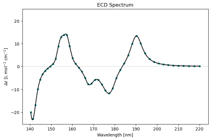
Text file
@jobs
task: response
@end

@method settings
basis: def2-svpd
xcfun: b3lyp
@end

@response
property: ecd (cpp)
# frequency region (and resolution)
frequencies:  0.207-0.325 (0.0025)
@end

@molecule
charge: 0
multiplicity: 1
xyz:
...
@end
Optical Rotatory Dispersion
The specific optical rotation can be determined directly from the complex polarization propagator evaluated for mixed electric- and magnetic-dipole operators Norman et al. (2004)Jiemchooroj & Norman (2007). In the current VeloxChem implementation, the isotropic optical-rotation parameter is defined as
where
and M is the molar mass. The mixed electric-magnetic dipole tensor, G′, is evaluated in the velocity gauge as given in the second expression, and is thereby gauge-origin independent. It is complex and calculated with a damping term, ℏγ, associated with the inverse finite lifetime of the excited states. The default program setting for this parameter is 0.124 eV (or 0.004556 a.u.).
This is the same mixed electric-dipole/magnetic-dipole response relation that underlies the Rosenfeld-style treatment of optical rotation Rosenfeld (1929)Norman et al. (2004), written here in the velocity gauge used by VeloxChem. When the molecular mass is available, the code converts β′(ω) in atomic units to specific rotation through
where νˉ is expressed in cm−1. The resulting values for [α]ω are reported in units of 103degdm−1(gcm−3)−1.
Python script
import numpy as np
import veloxchem as vlx

molecule = vlx.Molecule.read_xyz_string("""10

O             -1.009866880244         1.299407071912         1.951947754409
C              0.031038818173         2.001294498224         1.244371321259
C              0.339506903623         0.795807201271         2.029917688849
C              0.600316751832        -0.544462572436         1.394186918859
H             -0.026285836651         1.930258644799         0.154459855148
H              0.271804379347         2.990968281608         1.641505800108
H              0.794935917667         0.948100885444         3.014899839267
H              0.113110324011        -0.610670447580         0.412641743927
H              1.681576973773        -0.701096452623         1.264343536564
H              0.213803265264        -1.354101659046         2.029564064183""")

basis = vlx.MolecularBasis.read(molecule, "aug-cc-pvdz")

scf_drv = vlx.ScfRestrictedDriver()
scf_drv.xcfun = "b3lyp"
scf_results = scf_drv.compute(molecule, basis)

cpp_drv = vlx.ComplexResponse()
cpp_drv.frequencies = np.arange(0.207, 0.325, 0.0025)
cpp_drv.property = "ord"

cpp_results = cpp_drv.compute(molecule, basis, scf_results)
                                            Self Consistent Field Driver Setup
                                           ====================================

                   Wave Function Model             : Spin-Restricted Kohn-Sham
                   Initial Guess Model             : Superposition of Atomic Densities
                   Convergence Accelerator         : Two Level Direct Inversion of Iterative Subspace
                   Max. Number of Iterations       : 50
                   Max. Number of Error Vectors    : 10
                   Convergence Threshold           : 1.0e-06
                   ERI Screening Threshold         : 1.0e-12
                   Linear Dependence Threshold     : 1.0e-06
                   Exchange-Correlation Functional : B3LYP
                   Molecular Grid Level            : 4

* Info * Using the B3LYP functional.

         P. J. Stephens, F. J. Devlin, C. F. Chabalowski, and M. J. Frisch.,  J. Phys. Chem. 98, 11623 (1994)

* Info * Using the Libxc library (v7.0.0).

         S. Lehtola, C. Steigemann, M. J.T. Oliveira, and M. A.L. Marques.,  SoftwareX 7, 1–5 (2018)

* Info * Using the following algorithm for XC numerical integration.

         J. Kussmann, H. Laqua and C. Ochsenfeld, J. Chem. Theory Comput. 2021, 17, 1512-1521

* Info * Starting Reduced Basis SCF calculation...
* Info * ...done. SCF energy in reduced basis set: -191.823960423869 a.u. Time: 0.21 sec.


               Iter. |    Kohn-Sham Energy | Energy Change | Gradient Norm | Max. Gradient | Density Change
               --------------------------------------------------------------------------------------------
                  1      -193.118458872835    0.0000000000      0.37554496      0.01584480      0.00000000
                  2      -193.123363772890   -0.0049049001      0.31279732      0.01116367      0.35290190
                  3      -193.133247393175   -0.0098836203      0.09723785      0.00344749      0.19548399
                  4      -193.134034399260   -0.0007870061      0.02578568      0.00095366      0.03577760
                  5      -193.134110134095   -0.0000757348      0.00220004      0.00009796      0.01460491
                  6      -193.134110453180   -0.0000003191      0.00150842      0.00005205      0.00186854
                  7      -193.134110721512   -0.0000002683      0.00019811      0.00000712      0.00088667
                  8      -193.134110726432   -0.0000000049      0.00004901      0.00000196      0.00011428
                  9      -193.134110726716   -0.0000000003      0.00001349      0.00000071      0.00003271
                 10      -193.134110726738   -0.0000000000      0.00000258      0.00000012      0.00000770
                 11      -193.134110726739   -0.0000000000      0.00000033      0.00000002      0.00000182

               *** SCF converged in 11 iterations. Time: 3.75 sec.

               Spin-Restricted Kohn-Sham:
               --------------------------
               Total Energy                       :     -193.1341107267 a.u.
               Electronic Energy                  :     -317.2229127196 a.u.
               Nuclear Repulsion Energy           :      124.0888019929 a.u.
               ------------------------------------
               Gradient Norm                      :        0.0000003314 a.u.


               Ground State Information
               ------------------------
               Charge of Molecule            :  0.0
               Multiplicity (2S+1)           :  1
               Magnetic Quantum Number (M_S) :  0.0


                                              Complex Response Solver Setup
                                             ===============================

                               Number of Frequencies           : 48
                               Max. Number of Iterations       : 150
                               Convergence Threshold           : 1.0e-04
                               ERI Screening Threshold         : 1.0e-12
                               Exchange-Correlation Functional : B3LYP
                               Molecular Grid Level            : 4

* Info * Using the B3LYP functional.

         P. J. Stephens, F. J. Devlin, C. F. Chabalowski, and M. J. Frisch.,  J. Phys. Chem. 98, 11623 (1994)

* Info * Using the Libxc library (v7.0.0).

         S. Lehtola, C. Steigemann, M. J.T. Oliveira, and M. A.L. Marques.,  SoftwareX 7, 1–5 (2018)

* Info * Using the following algorithm for XC numerical integration.

         J. Kussmann, H. Laqua and C. Ochsenfeld, J. Chem. Theory Comput. 2021, 17, 1512-1521

* Info * 26 gerade trial vectors in reduced space
* Info * 25 ungerade trial vectors in reduced space

               *** Iteration:   1 * Residuals (Max,Min): 2.06e-01 and 8.84e-02

* Info * 57 gerade trial vectors in reduced space
* Info * 55 ungerade trial vectors in reduced space

               *** Iteration:   2 * Residuals (Max,Min): 3.87e-02 and 1.74e-02

* Info * 90 gerade trial vectors in reduced space
* Info * 87 ungerade trial vectors in reduced space

               *** Iteration:   3 * Residuals (Max,Min): 7.11e-03 and 1.99e-03

* Info * 122 gerade trial vectors in reduced space
* Info * 121 ungerade trial vectors in reduced space

               *** Iteration:   4 * Residuals (Max,Min): 1.04e-03 and 1.31e-04

* Info * 156 gerade trial vectors in reduced space
* Info * 153 ungerade trial vectors in reduced space

               *** Iteration:   5 * Residuals (Max,Min): 1.58e-04 and 7.00e-06

* Info * 164 gerade trial vectors in reduced space
* Info * 161 ungerade trial vectors in reduced space

               *** Iteration:   6 * Residuals (Max,Min): 9.21e-05 and 7.00e-06

               *** Complex response converged in 6 iterations. Time: 45.66 sec


               Optical Rotatory Dispersion Spectrum
               ====================================

     Frequency[a.u.]     Frequency[eV]       Optical rotatory dispersion [10$^3$ deg dm$^{-1}$ (g cm$^{-3}$)$^{-1}$]
     ---------------------------------------------------------------------------------------------------------------
               0.2070              5.63276                     2.28749510
               0.2095              5.70079                     2.73533850
               0.2120              5.76881                     3.28911186
               0.2145              5.83684                     3.98163918
               0.2170              5.90487                     4.85875325
               0.2195              5.97290                     5.98541278
               0.2220              6.04093                     7.45460926
               0.2245              6.10896                     9.39882389
               0.2270              6.17698                    11.99744022
               0.2295              6.24501                    15.44139887
               0.2320              6.31304                    19.65856595
               0.2345              6.38107                    22.85270588
               0.2370              6.44910                    15.65948896
               0.2395              6.51713                   -20.50503168
               0.2420              6.58516                   -59.76632726
               0.2445              6.65318                   -71.23122378
               0.2470              6.72121                   -72.17399456
               0.2495              6.78924                   -72.62159400
               0.2520              6.85727                   -72.03034043
               0.2545              6.92530                   -59.85991553
               0.2570              6.99333                   -29.26961551
               0.2595              7.06135                    -3.81984859
               0.2620              7.12938                     8.70866142
               0.2645              7.19741                     8.15493806
               0.2670              7.26544                     4.18694552
               0.2695              7.33347                     8.23610792
               0.2720              7.40150                    27.75833154
               0.2745              7.46953                    41.79267104
               0.2770              7.53755                    43.95606510
               0.2795              7.60558                    43.98022391
               0.2820              7.67361                    46.50679797
               0.2845              7.74164                    54.14310689
               0.2870              7.80967                    56.21094144
               0.2895              7.87770                    28.00920797
               0.2920              7.94572                    -5.77588004
               0.2945              8.01375                   -33.24006048
               0.2970              8.08178                   -65.20449275
               0.2995              8.14981                   -70.50822762
               0.3020              8.21784                   -64.47707634
               0.3045              8.28587                   -61.96822366
               0.3070              8.35390                   -62.59964821
               0.3095              8.42192                   -65.75559673
               0.3120              8.48995                   -71.39964314
               0.3145              8.55798                   -79.25244666
               0.3170              8.62601                   -86.35716747
               0.3195              8.69404                   -79.28100220
               0.3220              8.76207                   -31.54731360
               0.3245              8.83009                    27.24028283
cpp_drv.plot(cpp_results, x_unit='nm')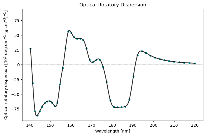
Text file
@jobs
task: response
@end

@method settings
basis: def2-svpd
xcfun: b3lyp
@end

@response
property: ord (cpp)
# frequency region (and resolution)
frequencies: 0.207-0.325 (0.0025)
@end

@molecule
charge: 0
multiplicity: 1
xyz:
...
@end
Exciton coupling model
VeloxChem implements the exciton coupling model (ECM) by Li et al. (2017) to determine circular dichroism spectra.
The ECM describes optical activity in molecular aggregates by representing the excited states of the full system in a reduced basis of localized monomer excitations and intermolecular charge-transfer (CT) configurations. In this framework, the electronic Hamiltonian is projected onto a subspace spanned by a user-defined number of excited states on each monomer, augmented by CT states constructed from selected occupied and virtual orbitals on neighboring units. The resulting excitonic Hamiltonian captures both Coulombic coupling between local excitations and explicit electron-hole transfer between monomers. Diagonalization of this Hamiltonian yields delocalized excited states from which rotatory strengths and circular dichroism spectra can be evaluated efficiently while retaining a clear connection to the underlying monomer electronic structure.
import math
from typing import List, Tuple

Atom = Tuple[str, float, float, float]


def build_ethylene_local(r_CC: float = 1.339, r_CH: float = 1.087) -> List[Atom]:
    """
    Construct a planar ethylene (C2H4) centered at the origin in the xy-plane.
    - C atoms placed at (-r_CC/2, 0, 0) and (+r_CC/2, 0, 0)
    - For each carbon, two hydrogens arranged trigonal-planar (120° apart),
      with the C-C bond being one of the three sp2 directions.

    Returns:
        List of (element, x, y, z) for 6 atoms: C, C, H, H, H, H
    """
    d = r_CC
    # Carbon positions
    c1 = (-d / 2.0, 0.0, 0.0)
    c2 = (d / 2.0, 0.0, 0.0)

    # Around C1: one bond to C2 at angle 0°; hydrogens at ±120° from +x
    ang1a = math.radians(120.0)
    ang1b = math.radians(-120.0)
    h1 = (c1[0] + r_CH * math.cos(ang1a), c1[1] + r_CH * math.sin(ang1a), 0.0)
    h2 = (c1[0] + r_CH * math.cos(ang1b), c1[1] + r_CH * math.sin(ang1b), 0.0)

    # Around C2: one bond to C1 at 180°; hydrogens at 180° ± 120° -> 60° and -60°
    ang2a = math.radians(60.0)
    ang2b = math.radians(-60.0)
    h3 = (c2[0] + r_CH * math.cos(ang2a), c2[1] + r_CH * math.sin(ang2a), 0.0)
    h4 = (c2[0] + r_CH * math.cos(ang2b), c2[1] + r_CH * math.sin(ang2b), 0.0)

    atoms = [
        ("C", *c1),
        ("C", *c2),
        ("H", *h1),
        ("H", *h2),
        ("H", *h3),
        ("H", *h4),
    ]
    return atoms


def rotate_z(x: float, y: float, z: float, phi: float) -> Tuple[float, float, float]:
    """
    Rotate a point around the z-axis by angle phi (radians).
    """
    c = math.cos(phi)
    s = math.sin(phi)
    xr = c * x - s * y
    yr = s * x + c * y
    return xr, yr, z


def build_stack(
    n_units: int,
    twist_deg: float,
    rise: float,
    radius: float,
    r_CC: float,
    r_CH: float,
) -> List[Atom]:
    """
    Build the full helical stack of ethylenes.

    Args:
        n_units: number of ethylene units
        twist_deg: twist angle per step (degrees)
        rise: translation along z per step (Å)
        radius: helix radius for the molecule centroids (Å)
        r_CC: C=C bond length (Å)
        r_CH: C–H bond length (Å)

    Returns:
        List of atoms for the whole stack.
    """
    base = build_ethylene_local(r_CC=r_CC, r_CH=r_CH)
    all_atoms: List[Atom] = []
    for k in range(n_units):
        phi = math.radians(k * twist_deg)
        # Helix center for unit k
        cx = radius * math.cos(phi)
        cy = radius * math.sin(phi)
        cz = k * rise

        for el, x, y, z in base:
            xr, yr, zr = rotate_z(x, y, z, phi)
            all_atoms.append((el, xr + cx, yr + cy, zr + cz))

    return all_atoms


atoms = build_stack(
    n_units=10,
    twist_deg=10,
    rise=3.5,
    radius=0,
    r_CC=1.339,
    r_CH=1.087,
)

mol_str = ""
for el, x, y, z in atoms:
    mol_str += f"{el:2s} {x:12.6f} {y:12.6f} {z:12.6f}\n"
import veloxchem as vlx
molecule = vlx.Molecule.read_str(mol_str)molecule.show()Figure: A helical stack of 10 ethylene molecules (or fragments).
Python script
import veloxchem as vlx

# the molecule object can be built from a molecular string listing all fragments
# in the helical stack and all atoms in each fragment
molecule = vlx.Molecule.read_str(mol_str)
basis = vlx.MolecularBasis.read(molecule, "def2-svp")

exciton_drv = vlx.ExcitonModelDriver()

exciton_drv.update_settings({"fragments": "10", "atoms_per_fragment": "6"})

exciton_drv.xcfun_label = "b3lyp"
exciton_drv.nstates = 1
exciton_drv.ct_nocc = 0
exciton_drv.ct_nvir = 0

exciton_results = exciton_drv.compute(molecule, basis)
+---------------------------------+
| Exciton Model |
+---------------------------------+
Total number of atoms: 60
Total number of monomers: 10
Total number of LE states: 10
Total number of CT states: 0
Monomer 1 has 6 atoms
Monomer 2 has 6 atoms
Monomer 3 has 6 atoms
Monomer 4 has 6 atoms
Monomer 5 has 6 atoms
Monomer 6 has 6 atoms
Monomer 7 has 6 atoms
Monomer 8 has 6 atoms
Monomer 9 has 6 atoms
Monomer 10 has 6 atoms
+-----------------------------+
| Monomer 1 |
+-----------------------------+
Molecular Geometry (Angstroms)
================================
Atom Coordinate X Coordinate Y Coordinate Z
C -0.669500000000 0.000000000000 0.000000000000
C 0.669500000000 0.000000000000 0.000000000000
H -1.213000000000 0.941370000000 0.000000000000
H -1.213000000000 -0.941370000000 0.000000000000
H 1.213000000000 0.941370000000 0.000000000000
H 1.213000000000 -0.941370000000 0.000000000000
Molecular charge : 0
Spin multiplicity : 1
Number of atoms : 6
Number of alpha electrons : 8
Number of beta electrons : 8
Molecular Basis (Atomic Basis)
================================
Basis: DEF2-SVP
Atom Contracted GTOs Primitive GTOs
C (3S,2P,1D) (7S,4P,1D)
H (2S,1P) (4S,1P)
Contracted Basis Functions : 48
Primitive Basis Functions : 76
Self Consistent Field Driver Setup
====================================
Wave Function Model : Spin-Restricted Hartree-Fock
Initial Guess Model : Superposition of Atomic Densities
Convergence Accelerator : Two Level Direct Inversion of Iterative Subspace
Max. Number of Iterations : 150
Max. Number of Error Vectors : 10
Convergence Threshold : 1.0e-06
ERI Screening Threshold : 1.0e-12
Linear Dependence Threshold : 1.0e-06
* Info * Starting Reduced Basis SCF calculation...
* Info * ...done. SCF energy in reduced basis set: -77.938309059200 a.u. Time: 0.04 sec.
Iter. | Hartree-Fock Energy | Energy Change | Gradient Norm | Max. Gradient | Density Change
--------------------------------------------------------------------------------------------
1 -77.975954854431 0.0000000000 0.09491381 0.01284101 0.00000000
2 -77.976919179664 -0.0009643252 0.01409900 0.00240013 0.02939923
3 -77.976944315473 -0.0000251358 0.00304062 0.00049876 0.00446192
4 -77.976946075229 -0.0000017598 0.00047293 0.00006811 0.00148728
5 -77.976946135434 -0.0000000602 0.00007520 0.00001487 0.00034433
6 -77.976946137269 -0.0000000018 0.00001119 0.00000240 0.00007026
7 -77.976946137307 -0.0000000000 0.00000087 0.00000014 0.00001027
*** SCF converged in 7 iterations. Time: 0.08 sec.
Spin-Restricted Hartree-Fock:
-----------------------------
Total Energy : -77.9769461373 a.u.
Electronic Energy : -111.2651443436 a.u.
Nuclear Repulsion Energy : 33.2881982063 a.u.
------------------------------------
Gradient Norm : 0.0000008749 a.u.
Ground State Information
------------------------
Charge of Molecule : 0.0
Multiplicity (2S+1) : 1
Magnetic Quantum Number (M_S) : 0.0
TDA Eigensolver Setup
=======================
Number of States : 1
Max. Number of Iterations : 100
Convergence Threshold : 1.0e-04
ERI Screening Threshold : 1.0e-12
*** Iteration: 1 * Reduced Space: 3 * Residues (Max,Min): 6.46e-02 and 6.46e-02
State 1: 0.34450384 a.u. Residual Norm: 0.06460075
*** Iteration: 2 * Reduced Space: 4 * Residues (Max,Min): 1.31e-02 and 1.31e-02
State 1: 0.33812045 a.u. Residual Norm: 0.01310675
*** Iteration: 3 * Reduced Space: 5 * Residues (Max,Min): 2.48e-03 and 2.48e-03
State 1: 0.33800273 a.u. Residual Norm: 0.00248352
*** Iteration: 4 * Reduced Space: 6 * Residues (Max,Min): 4.75e-04 and 4.75e-04
State 1: 0.33799509 a.u. Residual Norm: 0.00047497
*** Iteration: 5 * Reduced Space: 7 * Residues (Max,Min): 9.56e-05 and 9.56e-05
State 1: 0.33799502 a.u. Residual Norm: 0.00009564
*** 1 excited states converged in 5 iterations. Time: 0.08 sec
Electric Transition Dipole Moments (dipole length, a.u.)
--------------------------------------------------------
X Y Z
Excited State S1: -0.000000 0.000000 0.167524
Electric Transition Dipole Moments (dipole velocity, a.u.)
----------------------------------------------------------
X Y Z
Excited State S1: -0.000000 -0.000000 0.285571
Magnetic Transition Dipole Moments (a.u.)
-----------------------------------------
X Y Z
Excited State S1: -0.000000 -0.000000 -0.000000
One-Photon Absorption
---------------------
Excited State S1: 0.33799502 a.u. 9.19731 eV Osc.Str. 0.0063
Electronic Circular Dichroism
-----------------------------
Excited State S1: Rot.Str. -0.000000 a.u. -0.0000 [10**(-40) cgs]
Character of excitations:
Excited state 1
---------------
HOMO -> LUMO+1 0.9938
*** Time used in monomer calculation: 0.24 sec
+-----------------------------+
| Monomer 2 |
+-----------------------------+
Molecular Geometry (Angstroms)
================================
Atom Coordinate X Coordinate Y Coordinate Z
C -0.659329000000 -0.116257000000 3.500000000000
C 0.659329000000 0.116257000000 3.500000000000
H -1.358039000000 0.716433000000 3.500000000000
H -1.031105000000 -1.137703000000 3.500000000000
H 1.031105000000 1.137703000000 3.500000000000
H 1.358039000000 -0.716433000000 3.500000000000
Molecular charge : 0
Spin multiplicity : 1
Number of atoms : 6
Number of alpha electrons : 8
Number of beta electrons : 8
Molecular Basis (Atomic Basis)
================================
Basis: DEF2-SVP
Atom Contracted GTOs Primitive GTOs
C (3S,2P,1D) (7S,4P,1D)
H (2S,1P) (4S,1P)
Contracted Basis Functions : 48
Primitive Basis Functions : 76
Self Consistent Field Driver Setup
====================================
Wave Function Model : Spin-Restricted Hartree-Fock
Initial Guess Model : Superposition of Atomic Densities
Convergence Accelerator : Two Level Direct Inversion of Iterative Subspace
Max. Number of Iterations : 150
Max. Number of Error Vectors : 10
Convergence Threshold : 1.0e-06
ERI Screening Threshold : 1.0e-12
Linear Dependence Threshold : 1.0e-06
* Info * Starting Reduced Basis SCF calculation...
* Info * ...done. SCF energy in reduced basis set: -77.938309074802 a.u. Time: 0.02 sec.
Iter. | Hartree-Fock Energy | Energy Change | Gradient Norm | Max. Gradient | Density Change
--------------------------------------------------------------------------------------------
1 -77.975954864507 0.0000000000 0.09491381 0.01284100 0.00000000
2 -77.976919189339 -0.0009643248 0.01409898 0.00240013 0.02939920
3 -77.976944325074 -0.0000251357 0.00304061 0.00049876 0.00446192
4 -77.976946084825 -0.0000017598 0.00047292 0.00006811 0.00148728
5 -77.976946145030 -0.0000000602 0.00007520 0.00001487 0.00034433
6 -77.976946146865 -0.0000000018 0.00001119 0.00000240 0.00007026
7 -77.976946146903 -0.0000000000 0.00000087 0.00000014 0.00001027
*** SCF converged in 7 iterations. Time: 0.08 sec.
Spin-Restricted Hartree-Fock:
-----------------------------
Total Energy : -77.9769461469 a.u.
Electronic Energy : -111.2651463836 a.u.
Nuclear Repulsion Energy : 33.2882002367 a.u.
------------------------------------
Gradient Norm : 0.0000008749 a.u.
Ground State Information
------------------------
Charge of Molecule : 0.0
Multiplicity (2S+1) : 1
Magnetic Quantum Number (M_S) : 0.0
TDA Eigensolver Setup
=======================
Number of States : 1
Max. Number of Iterations : 100
Convergence Threshold : 1.0e-04
ERI Screening Threshold : 1.0e-12
*** Iteration: 1 * Reduced Space: 3 * Residues (Max,Min): 6.46e-02 and 6.46e-02
State 1: 0.34450387 a.u. Residual Norm: 0.06460071
*** Iteration: 2 * Reduced Space: 4 * Residues (Max,Min): 1.31e-02 and 1.31e-02
State 1: 0.33812049 a.u. Residual Norm: 0.01310673
*** Iteration: 3 * Reduced Space: 5 * Residues (Max,Min): 2.48e-03 and 2.48e-03
State 1: 0.33800278 a.u. Residual Norm: 0.00248352
*** Iteration: 4 * Reduced Space: 6 * Residues (Max,Min): 4.75e-04 and 4.75e-04
State 1: 0.33799513 a.u. Residual Norm: 0.00047497
*** Iteration: 5 * Reduced Space: 7 * Residues (Max,Min): 9.56e-05 and 9.56e-05
State 1: 0.33799506 a.u. Residual Norm: 0.00009564
*** 1 excited states converged in 5 iterations. Time: 0.07 sec
Electric Transition Dipole Moments (dipole length, a.u.)
--------------------------------------------------------
X Y Z
Excited State S1: 0.000000 0.000000 -0.167525
Electric Transition Dipole Moments (dipole velocity, a.u.)
----------------------------------------------------------
X Y Z
Excited State S1: 0.000000 0.000000 -0.285571
Magnetic Transition Dipole Moments (a.u.)
-----------------------------------------
X Y Z
Excited State S1: -0.000000 0.000000 0.000000
One-Photon Absorption
---------------------
Excited State S1: 0.33799506 a.u. 9.19731 eV Osc.Str. 0.0063
Electronic Circular Dichroism
-----------------------------
Excited State S1: Rot.Str. -0.000000 a.u. -0.0000 [10**(-40) cgs]
Character of excitations:
Excited state 1
---------------
HOMO -> LUMO+1 0.9938
*** Time used in monomer calculation: 0.20 sec
+-----------------------------+
| Monomer 3 |
+-----------------------------+
Molecular Geometry (Angstroms)
================================
Atom Coordinate X Coordinate Y Coordinate Z
C -0.629124000000 -0.228982000000 7.000000000000
C 0.629124000000 0.228982000000 7.000000000000
H -1.461815000000 0.469728000000 7.000000000000
H -0.817880000000 -1.299469000000 7.000000000000
H 0.817880000000 1.299469000000 7.000000000000
H 1.461815000000 -0.469728000000 7.000000000000
Molecular charge : 0
Spin multiplicity : 1
Number of atoms : 6
Number of alpha electrons : 8
Number of beta electrons : 8
Molecular Basis (Atomic Basis)
================================
Basis: DEF2-SVP
Atom Contracted GTOs Primitive GTOs
C (3S,2P,1D) (7S,4P,1D)
H (2S,1P) (4S,1P)
Contracted Basis Functions : 48
Primitive Basis Functions : 76
Self Consistent Field Driver Setup
====================================
Wave Function Model : Spin-Restricted Hartree-Fock
Initial Guess Model : Superposition of Atomic Densities
Convergence Accelerator : Two Level Direct Inversion of Iterative Subspace
Max. Number of Iterations : 150
Max. Number of Error Vectors : 10
Convergence Threshold : 1.0e-06
ERI Screening Threshold : 1.0e-12
Linear Dependence Threshold : 1.0e-06
* Info * Starting Reduced Basis SCF calculation...
* Info * ...done. SCF energy in reduced basis set: -77.938309088905 a.u. Time: 0.02 sec.
Iter. | Hartree-Fock Energy | Energy Change | Gradient Norm | Max. Gradient | Density Change
--------------------------------------------------------------------------------------------
1 -77.975954896236 0.0000000000 0.09491383 0.01284101 0.00000000
2 -77.976919222066 -0.0009643258 0.01409902 0.00240014 0.02939927
3 -77.976944357977 -0.0000251359 0.00304062 0.00049876 0.00446193
4 -77.976946117739 -0.0000017598 0.00047293 0.00006811 0.00148728
5 -77.976946177945 -0.0000000602 0.00007520 0.00001487 0.00034433
6 -77.976946179780 -0.0000000018 0.00001119 0.00000240 0.00007026
7 -77.976946179818 -0.0000000000 0.00000087 0.00000014 0.00001027
*** SCF converged in 7 iterations. Time: 0.08 sec.
Spin-Restricted Hartree-Fock:
-----------------------------
Total Energy : -77.9769461798 a.u.
Electronic Energy : -111.2651474926 a.u.
Nuclear Repulsion Energy : 33.2882013127 a.u.
------------------------------------
Gradient Norm : 0.0000008749 a.u.
Ground State Information
------------------------
Charge of Molecule : 0.0
Multiplicity (2S+1) : 1
Magnetic Quantum Number (M_S) : 0.0
TDA Eigensolver Setup
=======================
Number of States : 1
Max. Number of Iterations : 100
Convergence Threshold : 1.0e-04
ERI Screening Threshold : 1.0e-12
*** Iteration: 1 * Reduced Space: 3 * Residues (Max,Min): 6.46e-02 and 6.46e-02
State 1: 0.34450401 a.u. Residual Norm: 0.06460078
*** Iteration: 2 * Reduced Space: 4 * Residues (Max,Min): 1.31e-02 and 1.31e-02
State 1: 0.33812062 a.u. Residual Norm: 0.01310675
*** Iteration: 3 * Reduced Space: 5 * Residues (Max,Min): 2.48e-03 and 2.48e-03
State 1: 0.33800290 a.u. Residual Norm: 0.00248352
*** Iteration: 4 * Reduced Space: 6 * Residues (Max,Min): 4.75e-04 and 4.75e-04
State 1: 0.33799526 a.u. Residual Norm: 0.00047497
*** Iteration: 5 * Reduced Space: 7 * Residues (Max,Min): 9.56e-05 and 9.56e-05
State 1: 0.33799519 a.u. Residual Norm: 0.00009564
*** 1 excited states converged in 5 iterations. Time: 0.08 sec
Electric Transition Dipole Moments (dipole length, a.u.)
--------------------------------------------------------
X Y Z
Excited State S1: -0.000000 -0.000000 0.167524
Electric Transition Dipole Moments (dipole velocity, a.u.)
----------------------------------------------------------
X Y Z
Excited State S1: -0.000000 -0.000000 0.285571
Magnetic Transition Dipole Moments (a.u.)
-----------------------------------------
X Y Z
Excited State S1: 0.000000 -0.000000 0.000000
One-Photon Absorption
---------------------
Excited State S1: 0.33799519 a.u. 9.19732 eV Osc.Str. 0.0063
Electronic Circular Dichroism
-----------------------------
Excited State S1: Rot.Str. 0.000000 a.u. 0.0000 [10**(-40) cgs]
Character of excitations:
Excited state 1
---------------
HOMO -> LUMO+1 0.9938
*** Time used in monomer calculation: 0.21 sec
+-----------------------------+
| Monomer 4 |
+-----------------------------+
Molecular Geometry (Angstroms)
================================
Atom Coordinate X Coordinate Y Coordinate Z
C -0.579804000000 -0.334750000000 10.500000000000
C 0.579804000000 0.334750000000 10.500000000000
H -1.521174000000 0.208750000000 10.500000000000
H -0.579804000000 -1.421750000000 10.500000000000
H 0.579804000000 1.421750000000 10.500000000000
H 1.521174000000 -0.208750000000 10.500000000000
Molecular charge : 0
Spin multiplicity : 1
Number of atoms : 6
Number of alpha electrons : 8
Number of beta electrons : 8
Molecular Basis (Atomic Basis)
================================
Basis: DEF2-SVP
Atom Contracted GTOs Primitive GTOs
C (3S,2P,1D) (7S,4P,1D)
H (2S,1P) (4S,1P)
Contracted Basis Functions : 48
Primitive Basis Functions : 76
Self Consistent Field Driver Setup
====================================
Wave Function Model : Spin-Restricted Hartree-Fock
Initial Guess Model : Superposition of Atomic Densities
Convergence Accelerator : Two Level Direct Inversion of Iterative Subspace
Max. Number of Iterations : 150
Max. Number of Error Vectors : 10
Convergence Threshold : 1.0e-06
ERI Screening Threshold : 1.0e-12
Linear Dependence Threshold : 1.0e-06
* Info * Starting Reduced Basis SCF calculation...
* Info * ...done. SCF energy in reduced basis set: -77.938309075091 a.u. Time: 0.02 sec.
Iter. | Hartree-Fock Energy | Energy Change | Gradient Norm | Max. Gradient | Density Change
--------------------------------------------------------------------------------------------
1 -77.975954869896 0.0000000000 0.09491381 0.01284101 0.00000000
2 -77.976919195022 -0.0009643251 0.01409899 0.00240013 0.02939922
3 -77.976944330810 -0.0000251358 0.00304062 0.00049876 0.00446192
4 -77.976946090564 -0.0000017598 0.00047292 0.00006811 0.00148728
5 -77.976946150769 -0.0000000602 0.00007520 0.00001487 0.00034433
6 -77.976946152604 -0.0000000018 0.00001119 0.00000240 0.00007026
7 -77.976946152643 -0.0000000000 0.00000087 0.00000014 0.00001027
*** SCF converged in 7 iterations. Time: 0.08 sec.
Spin-Restricted Hartree-Fock:
-----------------------------
Total Energy : -77.9769461526 a.u.
Electronic Energy : -111.2651464041 a.u.
Nuclear Repulsion Energy : 33.2882002515 a.u.
------------------------------------
Gradient Norm : 0.0000008749 a.u.
Ground State Information
------------------------
Charge of Molecule : 0.0
Multiplicity (2S+1) : 1
Magnetic Quantum Number (M_S) : 0.0
TDA Eigensolver Setup
=======================
Number of States : 1
Max. Number of Iterations : 100
Convergence Threshold : 1.0e-04
ERI Screening Threshold : 1.0e-12
*** Iteration: 1 * Reduced Space: 3 * Residues (Max,Min): 6.46e-02 and 6.46e-02
State 1: 0.34450390 a.u. Residual Norm: 0.06460074
*** Iteration: 2 * Reduced Space: 4 * Residues (Max,Min): 1.31e-02 and 1.31e-02
State 1: 0.33812051 a.u. Residual Norm: 0.01310674
*** Iteration: 3 * Reduced Space: 5 * Residues (Max,Min): 2.48e-03 and 2.48e-03
State 1: 0.33800280 a.u. Residual Norm: 0.00248352
*** Iteration: 4 * Reduced Space: 6 * Residues (Max,Min): 4.75e-04 and 4.75e-04
State 1: 0.33799515 a.u. Residual Norm: 0.00047497
*** Iteration: 5 * Reduced Space: 7 * Residues (Max,Min): 9.56e-05 and 9.56e-05
State 1: 0.33799508 a.u. Residual Norm: 0.00009564
*** 1 excited states converged in 5 iterations. Time: 0.06 sec
Electric Transition Dipole Moments (dipole length, a.u.)
--------------------------------------------------------
X Y Z
Excited State S1: -0.000000 -0.000000 0.167524
Electric Transition Dipole Moments (dipole velocity, a.u.)
----------------------------------------------------------
X Y Z
Excited State S1: -0.000000 -0.000000 0.285571
Magnetic Transition Dipole Moments (a.u.)
-----------------------------------------
X Y Z
Excited State S1: 0.000000 -0.000000 -0.000000
One-Photon Absorption
---------------------
Excited State S1: 0.33799508 a.u. 9.19731 eV Osc.Str. 0.0063
Electronic Circular Dichroism
-----------------------------
Excited State S1: Rot.Str. -0.000000 a.u. -0.0000 [10**(-40) cgs]
Character of excitations:
Excited state 1
---------------
HOMO -> LUMO+1 0.9938
*** Time used in monomer calculation: 0.20 sec
+-----------------------------+
| Monomer 5 |
+-----------------------------+
Molecular Geometry (Angstroms)
================================
Atom Coordinate X Coordinate Y Coordinate Z
C -0.512867000000 -0.430346000000 14.000000000000
C 0.512867000000 0.430346000000 14.000000000000
H -1.534313000000 -0.058570000000 14.000000000000
H -0.324111000000 -1.500832000000 14.000000000000
H 0.324111000000 1.500832000000 14.000000000000
H 1.534313000000 0.058570000000 14.000000000000
Molecular charge : 0
Spin multiplicity : 1
Number of atoms : 6
Number of alpha electrons : 8
Number of beta electrons : 8
Molecular Basis (Atomic Basis)
================================
Basis: DEF2-SVP
Atom Contracted GTOs Primitive GTOs
C (3S,2P,1D) (7S,4P,1D)
H (2S,1P) (4S,1P)
Contracted Basis Functions : 48
Primitive Basis Functions : 76
Self Consistent Field Driver Setup
====================================
Wave Function Model : Spin-Restricted Hartree-Fock
Initial Guess Model : Superposition of Atomic Densities
Convergence Accelerator : Two Level Direct Inversion of Iterative Subspace
Max. Number of Iterations : 150
Max. Number of Error Vectors : 10
Convergence Threshold : 1.0e-06
ERI Screening Threshold : 1.0e-12
Linear Dependence Threshold : 1.0e-06
* Info * Starting Reduced Basis SCF calculation...
* Info * ...done. SCF energy in reduced basis set: -77.938309060757 a.u. Time: 0.02 sec.
Iter. | Hartree-Fock Energy | Energy Change | Gradient Norm | Max. Gradient | Density Change
--------------------------------------------------------------------------------------------
1 -77.975954858712 0.0000000000 0.09491381 0.01284100 0.00000000
2 -77.976919183838 -0.0009643251 0.01409899 0.00240013 0.02939922
3 -77.976944319627 -0.0000251358 0.00304062 0.00049876 0.00446192
4 -77.976946079381 -0.0000017598 0.00047292 0.00006811 0.00148728
5 -77.976946139586 -0.0000000602 0.00007520 0.00001487 0.00034433
6 -77.976946141421 -0.0000000018 0.00001119 0.00000240 0.00007026
7 -77.976946141459 -0.0000000000 0.00000087 0.00000014 0.00001027
*** SCF converged in 7 iterations. Time: 0.08 sec.
Spin-Restricted Hartree-Fock:
-----------------------------
Total Energy : -77.9769461415 a.u.
Electronic Energy : -111.2651479553 a.u.
Nuclear Repulsion Energy : 33.2882018138 a.u.
------------------------------------
Gradient Norm : 0.0000008749 a.u.
Ground State Information
------------------------
Charge of Molecule : 0.0
Multiplicity (2S+1) : 1
Magnetic Quantum Number (M_S) : 0.0
TDA Eigensolver Setup
=======================
Number of States : 1
Max. Number of Iterations : 100
Convergence Threshold : 1.0e-04
ERI Screening Threshold : 1.0e-12
*** Iteration: 1 * Reduced Space: 3 * Residues (Max,Min): 6.46e-02 and 6.46e-02
State 1: 0.34450386 a.u. Residual Norm: 0.06460074
*** Iteration: 2 * Reduced Space: 4 * Residues (Max,Min): 1.31e-02 and 1.31e-02
State 1: 0.33812048 a.u. Residual Norm: 0.01310674
*** Iteration: 3 * Reduced Space: 5 * Residues (Max,Min): 2.48e-03 and 2.48e-03
State 1: 0.33800276 a.u. Residual Norm: 0.00248352
*** Iteration: 4 * Reduced Space: 6 * Residues (Max,Min): 4.75e-04 and 4.75e-04
State 1: 0.33799512 a.u. Residual Norm: 0.00047497
*** Iteration: 5 * Reduced Space: 7 * Residues (Max,Min): 9.56e-05 and 9.56e-05
State 1: 0.33799505 a.u. Residual Norm: 0.00009564
*** 1 excited states converged in 5 iterations. Time: 0.07 sec
Electric Transition Dipole Moments (dipole length, a.u.)
--------------------------------------------------------
X Y Z
Excited State S1: -0.000000 -0.000000 -0.167524
Electric Transition Dipole Moments (dipole velocity, a.u.)
----------------------------------------------------------
X Y Z
Excited State S1: -0.000000 -0.000000 -0.285571
Magnetic Transition Dipole Moments (a.u.)
-----------------------------------------
X Y Z
Excited State S1: 0.000000 -0.000000 0.000000
One-Photon Absorption
---------------------
Excited State S1: 0.33799505 a.u. 9.19731 eV Osc.Str. 0.0063
Electronic Circular Dichroism
-----------------------------
Excited State S1: Rot.Str. -0.000000 a.u. -0.0000 [10**(-40) cgs]
Character of excitations:
Excited state 1
---------------
HOMO -> LUMO+1 -0.9938
*** Time used in monomer calculation: 0.21 sec
+-----------------------------+
| Monomer 6 |
+-----------------------------+
Molecular Geometry (Angstroms)
================================
Atom Coordinate X Coordinate Y Coordinate Z
C -0.430346000000 -0.512867000000 17.500000000000
C 0.430346000000 0.512867000000 17.500000000000
H -1.500832000000 -0.324111000000 17.500000000000
H -0.058570000000 -1.534313000000 17.500000000000
H 0.058570000000 1.534313000000 17.500000000000
H 1.500832000000 0.324111000000 17.500000000000
Molecular charge : 0
Spin multiplicity : 1
Number of atoms : 6
Number of alpha electrons : 8
Number of beta electrons : 8
Molecular Basis (Atomic Basis)
================================
Basis: DEF2-SVP
Atom Contracted GTOs Primitive GTOs
C (3S,2P,1D) (7S,4P,1D)
H (2S,1P) (4S,1P)
Contracted Basis Functions : 48
Primitive Basis Functions : 76
Self Consistent Field Driver Setup
====================================
Wave Function Model : Spin-Restricted Hartree-Fock
Initial Guess Model : Superposition of Atomic Densities
Convergence Accelerator : Two Level Direct Inversion of Iterative Subspace
Max. Number of Iterations : 150
Max. Number of Error Vectors : 10
Convergence Threshold : 1.0e-06
ERI Screening Threshold : 1.0e-12
Linear Dependence Threshold : 1.0e-06
* Info * Starting Reduced Basis SCF calculation...
* Info * ...done. SCF energy in reduced basis set: -77.938309060757 a.u. Time: 0.02 sec.
Iter. | Hartree-Fock Energy | Energy Change | Gradient Norm | Max. Gradient | Density Change
--------------------------------------------------------------------------------------------
1 -77.975954858712 0.0000000000 0.09491381 0.01284100 0.00000000
2 -77.976919183838 -0.0009643251 0.01409899 0.00240013 0.02939922
3 -77.976944319627 -0.0000251358 0.00304062 0.00049876 0.00446192
4 -77.976946079381 -0.0000017598 0.00047292 0.00006811 0.00148728
5 -77.976946139586 -0.0000000602 0.00007520 0.00001487 0.00034433
6 -77.976946141421 -0.0000000018 0.00001119 0.00000240 0.00007026
7 -77.976946141459 -0.0000000000 0.00000087 0.00000014 0.00001027
*** SCF converged in 7 iterations. Time: 0.07 sec.
Spin-Restricted Hartree-Fock:
-----------------------------
Total Energy : -77.9769461415 a.u.
Electronic Energy : -111.2651479553 a.u.
Nuclear Repulsion Energy : 33.2882018138 a.u.
------------------------------------
Gradient Norm : 0.0000008749 a.u.
Ground State Information
------------------------
Charge of Molecule : 0.0
Multiplicity (2S+1) : 1
Magnetic Quantum Number (M_S) : 0.0
TDA Eigensolver Setup
=======================
Number of States : 1
Max. Number of Iterations : 100
Convergence Threshold : 1.0e-04
ERI Screening Threshold : 1.0e-12
*** Iteration: 1 * Reduced Space: 3 * Residues (Max,Min): 6.46e-02 and 6.46e-02
State 1: 0.34450386 a.u. Residual Norm: 0.06460074
*** Iteration: 2 * Reduced Space: 4 * Residues (Max,Min): 1.31e-02 and 1.31e-02
State 1: 0.33812048 a.u. Residual Norm: 0.01310674
*** Iteration: 3 * Reduced Space: 5 * Residues (Max,Min): 2.48e-03 and 2.48e-03
State 1: 0.33800276 a.u. Residual Norm: 0.00248352
*** Iteration: 4 * Reduced Space: 6 * Residues (Max,Min): 4.75e-04 and 4.75e-04
State 1: 0.33799512 a.u. Residual Norm: 0.00047497
*** Iteration: 5 * Reduced Space: 7 * Residues (Max,Min): 9.56e-05 and 9.56e-05
State 1: 0.33799505 a.u. Residual Norm: 0.00009564
*** 1 excited states converged in 5 iterations. Time: 0.08 sec
Electric Transition Dipole Moments (dipole length, a.u.)
--------------------------------------------------------
X Y Z
Excited State S1: -0.000000 -0.000000 0.167524
Electric Transition Dipole Moments (dipole velocity, a.u.)
----------------------------------------------------------
X Y Z
Excited State S1: -0.000000 -0.000000 0.285571
Magnetic Transition Dipole Moments (a.u.)
-----------------------------------------
X Y Z
Excited State S1: 0.000000 -0.000000 0.000000
One-Photon Absorption
---------------------
Excited State S1: 0.33799505 a.u. 9.19731 eV Osc.Str. 0.0063
Electronic Circular Dichroism
-----------------------------
Excited State S1: Rot.Str. 0.000000 a.u. 0.0000 [10**(-40) cgs]
Character of excitations:
Excited state 1
---------------
HOMO -> LUMO+1 0.9938
*** Time used in monomer calculation: 0.21 sec
+-----------------------------+
| Monomer 7 |
+-----------------------------+
Molecular Geometry (Angstroms)
================================
Atom Coordinate X Coordinate Y Coordinate Z
C -0.334750000000 -0.579804000000 21.000000000000
C 0.334750000000 0.579804000000 21.000000000000
H -1.421750000000 -0.579804000000 21.000000000000
H 0.208750000000 -1.521174000000 21.000000000000
H -0.208750000000 1.521174000000 21.000000000000
H 1.421750000000 0.579804000000 21.000000000000
Molecular charge : 0
Spin multiplicity : 1
Number of atoms : 6
Number of alpha electrons : 8
Number of beta electrons : 8
Molecular Basis (Atomic Basis)
================================
Basis: DEF2-SVP
Atom Contracted GTOs Primitive GTOs
C (3S,2P,1D) (7S,4P,1D)
H (2S,1P) (4S,1P)
Contracted Basis Functions : 48
Primitive Basis Functions : 76
Self Consistent Field Driver Setup
====================================
Wave Function Model : Spin-Restricted Hartree-Fock
Initial Guess Model : Superposition of Atomic Densities
Convergence Accelerator : Two Level Direct Inversion of Iterative Subspace
Max. Number of Iterations : 150
Max. Number of Error Vectors : 10
Convergence Threshold : 1.0e-06
ERI Screening Threshold : 1.0e-12
Linear Dependence Threshold : 1.0e-06
* Info * Starting Reduced Basis SCF calculation...
* Info * ...done. SCF energy in reduced basis set: -77.938309075091 a.u. Time: 0.02 sec.
Iter. | Hartree-Fock Energy | Energy Change | Gradient Norm | Max. Gradient | Density Change
--------------------------------------------------------------------------------------------
1 -77.975954869896 0.0000000000 0.09491381 0.01284101 0.00000000
2 -77.976919195022 -0.0009643251 0.01409899 0.00240013 0.02939922
3 -77.976944330810 -0.0000251358 0.00304062 0.00049876 0.00446192
4 -77.976946090564 -0.0000017598 0.00047292 0.00006811 0.00148728
5 -77.976946150769 -0.0000000602 0.00007520 0.00001487 0.00034433
6 -77.976946152604 -0.0000000018 0.00001119 0.00000240 0.00007026
7 -77.976946152642 -0.0000000000 0.00000087 0.00000014 0.00001027
*** SCF converged in 7 iterations. Time: 0.08 sec.
Spin-Restricted Hartree-Fock:
-----------------------------
Total Energy : -77.9769461526 a.u.
Electronic Energy : -111.2651464041 a.u.
Nuclear Repulsion Energy : 33.2882002515 a.u.
------------------------------------
Gradient Norm : 0.0000008749 a.u.
Ground State Information
------------------------
Charge of Molecule : 0.0
Multiplicity (2S+1) : 1
Magnetic Quantum Number (M_S) : 0.0
TDA Eigensolver Setup
=======================
Number of States : 1
Max. Number of Iterations : 100
Convergence Threshold : 1.0e-04
ERI Screening Threshold : 1.0e-12
*** Iteration: 1 * Reduced Space: 3 * Residues (Max,Min): 6.46e-02 and 6.46e-02
State 1: 0.34450390 a.u. Residual Norm: 0.06460074
*** Iteration: 2 * Reduced Space: 4 * Residues (Max,Min): 1.31e-02 and 1.31e-02
State 1: 0.33812051 a.u. Residual Norm: 0.01310674
*** Iteration: 3 * Reduced Space: 5 * Residues (Max,Min): 2.48e-03 and 2.48e-03
State 1: 0.33800280 a.u. Residual Norm: 0.00248352
*** Iteration: 4 * Reduced Space: 6 * Residues (Max,Min): 4.75e-04 and 4.75e-04
State 1: 0.33799515 a.u. Residual Norm: 0.00047497
*** Iteration: 5 * Reduced Space: 7 * Residues (Max,Min): 9.56e-05 and 9.56e-05
State 1: 0.33799508 a.u. Residual Norm: 0.00009564
*** 1 excited states converged in 5 iterations. Time: 0.08 sec
Electric Transition Dipole Moments (dipole length, a.u.)
--------------------------------------------------------
X Y Z
Excited State S1: -0.000000 -0.000000 0.167524
Electric Transition Dipole Moments (dipole velocity, a.u.)
----------------------------------------------------------
X Y Z
Excited State S1: -0.000000 -0.000000 0.285571
Magnetic Transition Dipole Moments (a.u.)
-----------------------------------------
X Y Z
Excited State S1: 0.000000 -0.000000 0.000000
One-Photon Absorption
---------------------
Excited State S1: 0.33799508 a.u. 9.19731 eV Osc.Str. 0.0063
Electronic Circular Dichroism
-----------------------------
Excited State S1: Rot.Str. 0.000000 a.u. 0.0000 [10**(-40) cgs]
Character of excitations:
Excited state 1
---------------
HOMO -> LUMO+1 0.9938
*** Time used in monomer calculation: 0.22 sec
+-----------------------------+
| Monomer 8 |
+-----------------------------+
Molecular Geometry (Angstroms)
================================
Atom Coordinate X Coordinate Y Coordinate Z
C -0.228982000000 -0.629124000000 24.500000000000
C 0.228982000000 0.629124000000 24.500000000000
H -1.299469000000 -0.817880000000 24.500000000000
H 0.469728000000 -1.461815000000 24.500000000000
H -0.469728000000 1.461815000000 24.500000000000
H 1.299469000000 0.817880000000 24.500000000000
Molecular charge : 0
Spin multiplicity : 1
Number of atoms : 6
Number of alpha electrons : 8
Number of beta electrons : 8
Molecular Basis (Atomic Basis)
================================
Basis: DEF2-SVP
Atom Contracted GTOs Primitive GTOs
C (3S,2P,1D) (7S,4P,1D)
H (2S,1P) (4S,1P)
Contracted Basis Functions : 48
Primitive Basis Functions : 76
Self Consistent Field Driver Setup
====================================
Wave Function Model : Spin-Restricted Hartree-Fock
Initial Guess Model : Superposition of Atomic Densities
Convergence Accelerator : Two Level Direct Inversion of Iterative Subspace
Max. Number of Iterations : 150
Max. Number of Error Vectors : 10
Convergence Threshold : 1.0e-06
ERI Screening Threshold : 1.0e-12
Linear Dependence Threshold : 1.0e-06
* Info * Starting Reduced Basis SCF calculation...
* Info * ...done. SCF energy in reduced basis set: -77.938309088905 a.u. Time: 0.02 sec.
Iter. | Hartree-Fock Energy | Energy Change | Gradient Norm | Max. Gradient | Density Change
--------------------------------------------------------------------------------------------
1 -77.975954896236 0.0000000000 0.09491383 0.01284101 0.00000000
2 -77.976919222066 -0.0009643258 0.01409902 0.00240014 0.02939927
3 -77.976944357977 -0.0000251359 0.00304062 0.00049876 0.00446193
4 -77.976946117739 -0.0000017598 0.00047293 0.00006811 0.00148728
5 -77.976946177945 -0.0000000602 0.00007520 0.00001487 0.00034433
6 -77.976946179780 -0.0000000018 0.00001119 0.00000240 0.00007026
7 -77.976946179818 -0.0000000000 0.00000087 0.00000014 0.00001027
*** SCF converged in 7 iterations. Time: 0.08 sec.
Spin-Restricted Hartree-Fock:
-----------------------------
Total Energy : -77.9769461798 a.u.
Electronic Energy : -111.2651474926 a.u.
Nuclear Repulsion Energy : 33.2882013127 a.u.
------------------------------------
Gradient Norm : 0.0000008749 a.u.
Ground State Information
------------------------
Charge of Molecule : 0.0
Multiplicity (2S+1) : 1
Magnetic Quantum Number (M_S) : 0.0
TDA Eigensolver Setup
=======================
Number of States : 1
Max. Number of Iterations : 100
Convergence Threshold : 1.0e-04
ERI Screening Threshold : 1.0e-12
*** Iteration: 1 * Reduced Space: 3 * Residues (Max,Min): 6.46e-02 and 6.46e-02
State 1: 0.34450401 a.u. Residual Norm: 0.06460078
*** Iteration: 2 * Reduced Space: 4 * Residues (Max,Min): 1.31e-02 and 1.31e-02
State 1: 0.33812062 a.u. Residual Norm: 0.01310675
*** Iteration: 3 * Reduced Space: 5 * Residues (Max,Min): 2.48e-03 and 2.48e-03
State 1: 0.33800290 a.u. Residual Norm: 0.00248352
*** Iteration: 4 * Reduced Space: 6 * Residues (Max,Min): 4.75e-04 and 4.75e-04
State 1: 0.33799526 a.u. Residual Norm: 0.00047497
*** Iteration: 5 * Reduced Space: 7 * Residues (Max,Min): 9.56e-05 and 9.56e-05
State 1: 0.33799519 a.u. Residual Norm: 0.00009564
*** 1 excited states converged in 5 iterations. Time: 0.08 sec
Electric Transition Dipole Moments (dipole length, a.u.)
--------------------------------------------------------
X Y Z
Excited State S1: 0.000000 0.000000 -0.167524
Electric Transition Dipole Moments (dipole velocity, a.u.)
----------------------------------------------------------
X Y Z
Excited State S1: 0.000000 0.000000 -0.285571
Magnetic Transition Dipole Moments (a.u.)
-----------------------------------------
X Y Z
Excited State S1: -0.000000 0.000000 0.000000
One-Photon Absorption
---------------------
Excited State S1: 0.33799519 a.u. 9.19732 eV Osc.Str. 0.0063
Electronic Circular Dichroism
-----------------------------
Excited State S1: Rot.Str. -0.000000 a.u. -0.0000 [10**(-40) cgs]
Character of excitations:
Excited state 1
---------------
HOMO -> LUMO+1 0.9938
*** Time used in monomer calculation: 0.22 sec
+-----------------------------+
| Monomer 9 |
+-----------------------------+
Molecular Geometry (Angstroms)
================================
Atom Coordinate X Coordinate Y Coordinate Z
C -0.116257000000 -0.659329000000 28.000000000000
C 0.116257000000 0.659329000000 28.000000000000
H -1.137703000000 -1.031105000000 28.000000000000
H 0.716433000000 -1.358039000000 28.000000000000
H -0.716433000000 1.358039000000 28.000000000000
H 1.137703000000 1.031105000000 28.000000000000
Molecular charge : 0
Spin multiplicity : 1
Number of atoms : 6
Number of alpha electrons : 8
Number of beta electrons : 8
Molecular Basis (Atomic Basis)
================================
Basis: DEF2-SVP
Atom Contracted GTOs Primitive GTOs
C (3S,2P,1D) (7S,4P,1D)
H (2S,1P) (4S,1P)
Contracted Basis Functions : 48
Primitive Basis Functions : 76
Self Consistent Field Driver Setup
====================================
Wave Function Model : Spin-Restricted Hartree-Fock
Initial Guess Model : Superposition of Atomic Densities
Convergence Accelerator : Two Level Direct Inversion of Iterative Subspace
Max. Number of Iterations : 150
Max. Number of Error Vectors : 10
Convergence Threshold : 1.0e-06
ERI Screening Threshold : 1.0e-12
Linear Dependence Threshold : 1.0e-06
* Info * Starting Reduced Basis SCF calculation...
* Info * ...done. SCF energy in reduced basis set: -77.938309074802 a.u. Time: 0.02 sec.
Iter. | Hartree-Fock Energy | Energy Change | Gradient Norm | Max. Gradient | Density Change
--------------------------------------------------------------------------------------------
1 -77.975954864507 0.0000000000 0.09491381 0.01284100 0.00000000
2 -77.976919189339 -0.0009643248 0.01409898 0.00240013 0.02939920
3 -77.976944325074 -0.0000251357 0.00304061 0.00049876 0.00446192
4 -77.976946084825 -0.0000017598 0.00047292 0.00006811 0.00148728
5 -77.976946145030 -0.0000000602 0.00007520 0.00001487 0.00034433
6 -77.976946146865 -0.0000000018 0.00001119 0.00000240 0.00007026
7 -77.976946146903 -0.0000000000 0.00000087 0.00000014 0.00001027
*** SCF converged in 7 iterations. Time: 0.09 sec.
Spin-Restricted Hartree-Fock:
-----------------------------
Total Energy : -77.9769461469 a.u.
Electronic Energy : -111.2651463836 a.u.
Nuclear Repulsion Energy : 33.2882002367 a.u.
------------------------------------
Gradient Norm : 0.0000008749 a.u.
Ground State Information
------------------------
Charge of Molecule : 0.0
Multiplicity (2S+1) : 1
Magnetic Quantum Number (M_S) : 0.0
TDA Eigensolver Setup
=======================
Number of States : 1
Max. Number of Iterations : 100
Convergence Threshold : 1.0e-04
ERI Screening Threshold : 1.0e-12
*** Iteration: 1 * Reduced Space: 3 * Residues (Max,Min): 6.46e-02 and 6.46e-02
State 1: 0.34450387 a.u. Residual Norm: 0.06460071
*** Iteration: 2 * Reduced Space: 4 * Residues (Max,Min): 1.31e-02 and 1.31e-02
State 1: 0.33812049 a.u. Residual Norm: 0.01310673
*** Iteration: 3 * Reduced Space: 5 * Residues (Max,Min): 2.48e-03 and 2.48e-03
State 1: 0.33800278 a.u. Residual Norm: 0.00248352
*** Iteration: 4 * Reduced Space: 6 * Residues (Max,Min): 4.75e-04 and 4.75e-04
State 1: 0.33799513 a.u. Residual Norm: 0.00047497
*** Iteration: 5 * Reduced Space: 7 * Residues (Max,Min): 9.56e-05 and 9.56e-05
State 1: 0.33799506 a.u. Residual Norm: 0.00009564
*** 1 excited states converged in 5 iterations. Time: 0.12 sec
Electric Transition Dipole Moments (dipole length, a.u.)
--------------------------------------------------------
X Y Z
Excited State S1: 0.000000 0.000000 -0.167525
Electric Transition Dipole Moments (dipole velocity, a.u.)
----------------------------------------------------------
X Y Z
Excited State S1: 0.000000 0.000000 -0.285571
Magnetic Transition Dipole Moments (a.u.)
-----------------------------------------
X Y Z
Excited State S1: -0.000000 0.000000 0.000000
One-Photon Absorption
---------------------
Excited State S1: 0.33799506 a.u. 9.19731 eV Osc.Str. 0.0063
Electronic Circular Dichroism
-----------------------------
Excited State S1: Rot.Str. -0.000000 a.u. -0.0000 [10**(-40) cgs]
Character of excitations:
Excited state 1
---------------
HOMO -> LUMO+1 0.9938
*** Time used in monomer calculation: 0.26 sec
+------------------------------+
| Monomer 10 |
+------------------------------+
Molecular Geometry (Angstroms)
================================
Atom Coordinate X Coordinate Y Coordinate Z
C -0.000000000000 -0.669500000000 31.500000000000
C 0.000000000000 0.669500000000 31.500000000000
H -0.941370000000 -1.213000000000 31.500000000000
H 0.941370000000 -1.213000000000 31.500000000000
H -0.941370000000 1.213000000000 31.500000000000
H 0.941370000000 1.213000000000 31.500000000000
Molecular charge : 0
Spin multiplicity : 1
Number of atoms : 6
Number of alpha electrons : 8
Number of beta electrons : 8
Molecular Basis (Atomic Basis)
================================
Basis: DEF2-SVP
Atom Contracted GTOs Primitive GTOs
C (3S,2P,1D) (7S,4P,1D)
H (2S,1P) (4S,1P)
Contracted Basis Functions : 48
Primitive Basis Functions : 76
Self Consistent Field Driver Setup
====================================
Wave Function Model : Spin-Restricted Hartree-Fock
Initial Guess Model : Superposition of Atomic Densities
Convergence Accelerator : Two Level Direct Inversion of Iterative Subspace
Max. Number of Iterations : 150
Max. Number of Error Vectors : 10
Convergence Threshold : 1.0e-06
ERI Screening Threshold : 1.0e-12
Linear Dependence Threshold : 1.0e-06
* Info * Starting Reduced Basis SCF calculation...
* Info * ...done. SCF energy in reduced basis set: -77.938309059200 a.u. Time: 0.02 sec.
Iter. | Hartree-Fock Energy | Energy Change | Gradient Norm | Max. Gradient | Density Change
--------------------------------------------------------------------------------------------
1 -77.975954854431 0.0000000000 0.09491381 0.01284101 0.00000000
2 -77.976919179664 -0.0009643252 0.01409900 0.00240013 0.02939923
3 -77.976944315473 -0.0000251358 0.00304062 0.00049876 0.00446192
4 -77.976946075229 -0.0000017598 0.00047293 0.00006811 0.00148728
5 -77.976946135434 -0.0000000602 0.00007520 0.00001487 0.00034433
6 -77.976946137269 -0.0000000018 0.00001119 0.00000240 0.00007026
7 -77.976946137307 -0.0000000000 0.00000087 0.00000014 0.00001027
*** SCF converged in 7 iterations. Time: 0.07 sec.
Spin-Restricted Hartree-Fock:
-----------------------------
Total Energy : -77.9769461373 a.u.
Electronic Energy : -111.2651443436 a.u.
Nuclear Repulsion Energy : 33.2881982063 a.u.
------------------------------------
Gradient Norm : 0.0000008749 a.u.
Ground State Information
------------------------
Charge of Molecule : 0.0
Multiplicity (2S+1) : 1
Magnetic Quantum Number (M_S) : 0.0
TDA Eigensolver Setup
=======================
Number of States : 1
Max. Number of Iterations : 100
Convergence Threshold : 1.0e-04
ERI Screening Threshold : 1.0e-12
*** Iteration: 1 * Reduced Space: 3 * Residues (Max,Min): 6.46e-02 and 6.46e-02
State 1: 0.34450384 a.u. Residual Norm: 0.06460075
*** Iteration: 2 * Reduced Space: 4 * Residues (Max,Min): 1.31e-02 and 1.31e-02
State 1: 0.33812045 a.u. Residual Norm: 0.01310675
*** Iteration: 3 * Reduced Space: 5 * Residues (Max,Min): 2.48e-03 and 2.48e-03
State 1: 0.33800273 a.u. Residual Norm: 0.00248352
*** Iteration: 4 * Reduced Space: 6 * Residues (Max,Min): 4.75e-04 and 4.75e-04
State 1: 0.33799509 a.u. Residual Norm: 0.00047497
*** Iteration: 5 * Reduced Space: 7 * Residues (Max,Min): 9.56e-05 and 9.56e-05
State 1: 0.33799502 a.u. Residual Norm: 0.00009564
*** 1 excited states converged in 5 iterations. Time: 0.08 sec
Electric Transition Dipole Moments (dipole length, a.u.)
--------------------------------------------------------
X Y Z
Excited State S1: -0.000000 -0.000000 0.167524
Electric Transition Dipole Moments (dipole velocity, a.u.)
----------------------------------------------------------
X Y Z
Excited State S1: -0.000000 -0.000000 0.285571
Magnetic Transition Dipole Moments (a.u.)
-----------------------------------------
X Y Z
Excited State S1: 0.000000 0.000000 -0.000000
One-Photon Absorption
---------------------
Excited State S1: 0.33799502 a.u. 9.19731 eV Osc.Str. 0.0063
Electronic Circular Dichroism
-----------------------------
Excited State S1: Rot.Str. -0.000000 a.u. -0.0000 [10**(-40) cgs]
Character of excitations:
Excited state 1
---------------
HOMO -> LUMO+1 0.9938
*** Time used in monomer calculation: 0.21 sec
+-----------------------------+
| Dimer 1 2 |
+-----------------------------+
Molecular Geometry (Angstroms)
================================
Atom Coordinate X Coordinate Y Coordinate Z
C -0.669500000000 0.000000000000 0.000000000000
C 0.669500000000 0.000000000000 0.000000000000
H -1.213000000000 0.941370000000 0.000000000000
H -1.213000000000 -0.941370000000 0.000000000000
H 1.213000000000 0.941370000000 0.000000000000
H 1.213000000000 -0.941370000000 0.000000000000
C -0.659329000000 -0.116257000000 3.500000000000
C 0.659329000000 0.116257000000 3.500000000000
H -1.358039000000 0.716433000000 3.500000000000
H -1.031105000000 -1.137703000000 3.500000000000
H 1.031105000000 1.137703000000 3.500000000000
H 1.358039000000 -0.716433000000 3.500000000000
Molecular charge : 0
Spin multiplicity : 1
Number of atoms : 12
Number of alpha electrons : 16
Number of beta electrons : 16
Molecular Basis (Atomic Basis)
================================
Basis: DEF2-SVP
Atom Contracted GTOs Primitive GTOs
C (3S,2P,1D) (7S,4P,1D)
H (2S,1P) (4S,1P)
Contracted Basis Functions : 96
Primitive Basis Functions : 152
Excitonic Couplings
=====================
Dimer Energy: -155.9600619781 a.u.
LE-LE coupling: 1e(1) 2e(1) -0.000955362564
*** Time used in dimer calculation: 0.15 sec
+-----------------------------+
| Dimer 1 3 |
+-----------------------------+
Molecular Geometry (Angstroms)
================================
Atom Coordinate X Coordinate Y Coordinate Z
C -0.669500000000 0.000000000000 0.000000000000
C 0.669500000000 0.000000000000 0.000000000000
H -1.213000000000 0.941370000000 0.000000000000
H -1.213000000000 -0.941370000000 0.000000000000
H 1.213000000000 0.941370000000 0.000000000000
H 1.213000000000 -0.941370000000 0.000000000000
C -0.629124000000 -0.228982000000 7.000000000000
C 0.629124000000 0.228982000000 7.000000000000
H -1.461815000000 0.469728000000 7.000000000000
H -0.817880000000 -1.299469000000 7.000000000000
H 0.817880000000 1.299469000000 7.000000000000
H 1.461815000000 -0.469728000000 7.000000000000
Molecular charge : 0
Spin multiplicity : 1
Number of atoms : 12
Number of alpha electrons : 16
Number of beta electrons : 16
Molecular Basis (Atomic Basis)
================================
Basis: DEF2-SVP
Atom Contracted GTOs Primitive GTOs
C (3S,2P,1D) (7S,4P,1D)
H (2S,1P) (4S,1P)
Contracted Basis Functions : 96
Primitive Basis Functions : 152
Excitonic Couplings
=====================
Dimer Energy: -155.9538177440 a.u.
LE-LE coupling: 1e(1) 3e(1) -0.000016212974
*** Time used in dimer calculation: 0.08 sec
+-----------------------------+
| Dimer 2 3 |
+-----------------------------+
Molecular Geometry (Angstroms)
================================
Atom Coordinate X Coordinate Y Coordinate Z
C -0.659329000000 -0.116257000000 3.500000000000
C 0.659329000000 0.116257000000 3.500000000000
H -1.358039000000 0.716433000000 3.500000000000
H -1.031105000000 -1.137703000000 3.500000000000
H 1.031105000000 1.137703000000 3.500000000000
H 1.358039000000 -0.716433000000 3.500000000000
C -0.629124000000 -0.228982000000 7.000000000000
C 0.629124000000 0.228982000000 7.000000000000
H -1.461815000000 0.469728000000 7.000000000000
H -0.817880000000 -1.299469000000 7.000000000000
H 0.817880000000 1.299469000000 7.000000000000
H 1.461815000000 -0.469728000000 7.000000000000
Molecular charge : 0
Spin multiplicity : 1
Number of atoms : 12
Number of alpha electrons : 16
Number of beta electrons : 16
Molecular Basis (Atomic Basis)
================================
Basis: DEF2-SVP
Atom Contracted GTOs Primitive GTOs
C (3S,2P,1D) (7S,4P,1D)
H (2S,1P) (4S,1P)
Contracted Basis Functions : 96
Primitive Basis Functions : 152
Excitonic Couplings
=====================
Dimer Energy: -155.9600620182 a.u.
LE-LE coupling: 2e(1) 3e(1) -0.000955362152
*** Time used in dimer calculation: 0.17 sec
+-----------------------------+
| Dimer 2 4 |
+-----------------------------+
Molecular Geometry (Angstroms)
================================
Atom Coordinate X Coordinate Y Coordinate Z
C -0.659329000000 -0.116257000000 3.500000000000
C 0.659329000000 0.116257000000 3.500000000000
H -1.358039000000 0.716433000000 3.500000000000
H -1.031105000000 -1.137703000000 3.500000000000
H 1.031105000000 1.137703000000 3.500000000000
H 1.358039000000 -0.716433000000 3.500000000000
C -0.579804000000 -0.334750000000 10.500000000000
C 0.579804000000 0.334750000000 10.500000000000
H -1.521174000000 0.208750000000 10.500000000000
H -0.579804000000 -1.421750000000 10.500000000000
H 0.579804000000 1.421750000000 10.500000000000
H 1.521174000000 -0.208750000000 10.500000000000
Molecular charge : 0
Spin multiplicity : 1
Number of atoms : 12
Number of alpha electrons : 16
Number of beta electrons : 16
Molecular Basis (Atomic Basis)
================================
Basis: DEF2-SVP
Atom Contracted GTOs Primitive GTOs
C (3S,2P,1D) (7S,4P,1D)
H (2S,1P) (4S,1P)
Contracted Basis Functions : 96
Primitive Basis Functions : 152
Excitonic Couplings
=====================
Dimer Energy: -155.9538177264 a.u.
LE-LE coupling: 2e(1) 4e(1) 0.000016213083
*** Time used in dimer calculation: 0.08 sec
+-----------------------------+
| Dimer 3 4 |
+-----------------------------+
Molecular Geometry (Angstroms)
================================
Atom Coordinate X Coordinate Y Coordinate Z
C -0.629124000000 -0.228982000000 7.000000000000
C 0.629124000000 0.228982000000 7.000000000000
H -1.461815000000 0.469728000000 7.000000000000
H -0.817880000000 -1.299469000000 7.000000000000
H 0.817880000000 1.299469000000 7.000000000000
H 1.461815000000 -0.469728000000 7.000000000000
C -0.579804000000 -0.334750000000 10.500000000000
C 0.579804000000 0.334750000000 10.500000000000
H -1.521174000000 0.208750000000 10.500000000000
H -0.579804000000 -1.421750000000 10.500000000000
H 0.579804000000 1.421750000000 10.500000000000
H 1.521174000000 -0.208750000000 10.500000000000
Molecular charge : 0
Spin multiplicity : 1
Number of atoms : 12
Number of alpha electrons : 16
Number of beta electrons : 16
Molecular Basis (Atomic Basis)
================================
Basis: DEF2-SVP
Atom Contracted GTOs Primitive GTOs
C (3S,2P,1D) (7S,4P,1D)
H (2S,1P) (4S,1P)
Contracted Basis Functions : 96
Primitive Basis Functions : 152
Excitonic Couplings
=====================
Dimer Energy: -155.9600620233 a.u.
LE-LE coupling: 3e(1) 4e(1) 0.000955361829
*** Time used in dimer calculation: 0.20 sec
+-----------------------------+
| Dimer 3 5 |
+-----------------------------+
Molecular Geometry (Angstroms)
================================
Atom Coordinate X Coordinate Y Coordinate Z
C -0.629124000000 -0.228982000000 7.000000000000
C 0.629124000000 0.228982000000 7.000000000000
H -1.461815000000 0.469728000000 7.000000000000
H -0.817880000000 -1.299469000000 7.000000000000
H 0.817880000000 1.299469000000 7.000000000000
H 1.461815000000 -0.469728000000 7.000000000000
C -0.512867000000 -0.430346000000 14.000000000000
C 0.512867000000 0.430346000000 14.000000000000
H -1.534313000000 -0.058570000000 14.000000000000
H -0.324111000000 -1.500832000000 14.000000000000
H 0.324111000000 1.500832000000 14.000000000000
H 1.534313000000 0.058570000000 14.000000000000
Molecular charge : 0
Spin multiplicity : 1
Number of atoms : 12
Number of alpha electrons : 16
Number of beta electrons : 16
Molecular Basis (Atomic Basis)
================================
Basis: DEF2-SVP
Atom Contracted GTOs Primitive GTOs
C (3S,2P,1D) (7S,4P,1D)
H (2S,1P) (4S,1P)
Contracted Basis Functions : 96
Primitive Basis Functions : 152
Excitonic Couplings
=====================
Dimer Energy: -155.9538177482 a.u.
LE-LE coupling: 3e(1) 5e(1) 0.000016212995
*** Time used in dimer calculation: 0.17 sec
+-----------------------------+
| Dimer 4 5 |
+-----------------------------+
Molecular Geometry (Angstroms)
================================
Atom Coordinate X Coordinate Y Coordinate Z
C -0.579804000000 -0.334750000000 10.500000000000
C 0.579804000000 0.334750000000 10.500000000000
H -1.521174000000 0.208750000000 10.500000000000
H -0.579804000000 -1.421750000000 10.500000000000
H 0.579804000000 1.421750000000 10.500000000000
H 1.521174000000 -0.208750000000 10.500000000000
C -0.512867000000 -0.430346000000 14.000000000000
C 0.512867000000 0.430346000000 14.000000000000
H -1.534313000000 -0.058570000000 14.000000000000
H -0.324111000000 -1.500832000000 14.000000000000
H 0.324111000000 1.500832000000 14.000000000000
H 1.534313000000 0.058570000000 14.000000000000
Molecular charge : 0
Spin multiplicity : 1
Number of atoms : 12
Number of alpha electrons : 16
Number of beta electrons : 16
Molecular Basis (Atomic Basis)
================================
Basis: DEF2-SVP
Atom Contracted GTOs Primitive GTOs
C (3S,2P,1D) (7S,4P,1D)
H (2S,1P) (4S,1P)
Contracted Basis Functions : 96
Primitive Basis Functions : 152
Excitonic Couplings
=====================
Dimer Energy: -155.9600619872 a.u.
LE-LE coupling: 4e(1) 5e(1) -0.000955362419
*** Time used in dimer calculation: 0.17 sec
+-----------------------------+
| Dimer 4 6 |
+-----------------------------+
Molecular Geometry (Angstroms)
================================
Atom Coordinate X Coordinate Y Coordinate Z
C -0.579804000000 -0.334750000000 10.500000000000
C 0.579804000000 0.334750000000 10.500000000000
H -1.521174000000 0.208750000000 10.500000000000
H -0.579804000000 -1.421750000000 10.500000000000
H 0.579804000000 1.421750000000 10.500000000000
H 1.521174000000 -0.208750000000 10.500000000000
C -0.430346000000 -0.512867000000 17.500000000000
C 0.430346000000 0.512867000000 17.500000000000
H -1.500832000000 -0.324111000000 17.500000000000
H -0.058570000000 -1.534313000000 17.500000000000
H 0.058570000000 1.534313000000 17.500000000000
H 1.500832000000 0.324111000000 17.500000000000
Molecular charge : 0
Spin multiplicity : 1
Number of atoms : 12
Number of alpha electrons : 16
Number of beta electrons : 16
Molecular Basis (Atomic Basis)
================================
Basis: DEF2-SVP
Atom Contracted GTOs Primitive GTOs
C (3S,2P,1D) (7S,4P,1D)
H (2S,1P) (4S,1P)
Contracted Basis Functions : 96
Primitive Basis Functions : 152
Excitonic Couplings
=====================
Dimer Energy: -155.9538177210 a.u.
LE-LE coupling: 4e(1) 6e(1) -0.000016213050
*** Time used in dimer calculation: 0.09 sec
+-----------------------------+
| Dimer 5 6 |
+-----------------------------+
Molecular Geometry (Angstroms)
================================
Atom Coordinate X Coordinate Y Coordinate Z
C -0.512867000000 -0.430346000000 14.000000000000
C 0.512867000000 0.430346000000 14.000000000000
H -1.534313000000 -0.058570000000 14.000000000000
H -0.324111000000 -1.500832000000 14.000000000000
H 0.324111000000 1.500832000000 14.000000000000
H 1.534313000000 0.058570000000 14.000000000000
C -0.430346000000 -0.512867000000 17.500000000000
C 0.430346000000 0.512867000000 17.500000000000
H -1.500832000000 -0.324111000000 17.500000000000
H -0.058570000000 -1.534313000000 17.500000000000
H 0.058570000000 1.534313000000 17.500000000000
H 1.500832000000 0.324111000000 17.500000000000
Molecular charge : 0
Spin multiplicity : 1
Number of atoms : 12
Number of alpha electrons : 16
Number of beta electrons : 16
Molecular Basis (Atomic Basis)
================================
Basis: DEF2-SVP
Atom Contracted GTOs Primitive GTOs
C (3S,2P,1D) (7S,4P,1D)
H (2S,1P) (4S,1P)
Contracted Basis Functions : 96
Primitive Basis Functions : 152
Excitonic Couplings
=====================
Dimer Energy: -155.9600619759 a.u.
LE-LE coupling: 5e(1) 6e(1) -0.000955362200
*** Time used in dimer calculation: 0.14 sec
+-----------------------------+
| Dimer 5 7 |
+-----------------------------+
Molecular Geometry (Angstroms)
================================
Atom Coordinate X Coordinate Y Coordinate Z
C -0.512867000000 -0.430346000000 14.000000000000
C 0.512867000000 0.430346000000 14.000000000000
H -1.534313000000 -0.058570000000 14.000000000000
H -0.324111000000 -1.500832000000 14.000000000000
H 0.324111000000 1.500832000000 14.000000000000
H 1.534313000000 0.058570000000 14.000000000000
C -0.334750000000 -0.579804000000 21.000000000000
C 0.334750000000 0.579804000000 21.000000000000
H -1.421750000000 -0.579804000000 21.000000000000
H 0.208750000000 -1.521174000000 21.000000000000
H -0.208750000000 1.521174000000 21.000000000000
H 1.421750000000 0.579804000000 21.000000000000
Molecular charge : 0
Spin multiplicity : 1
Number of atoms : 12
Number of alpha electrons : 16
Number of beta electrons : 16
Molecular Basis (Atomic Basis)
================================
Basis: DEF2-SVP
Atom Contracted GTOs Primitive GTOs
C (3S,2P,1D) (7S,4P,1D)
H (2S,1P) (4S,1P)
Contracted Basis Functions : 96
Primitive Basis Functions : 152
Excitonic Couplings
=====================
Dimer Energy: -155.9538177210 a.u.
LE-LE coupling: 5e(1) 7e(1) 0.000016213050
*** Time used in dimer calculation: 0.10 sec
+-----------------------------+
| Dimer 6 7 |
+-----------------------------+
Molecular Geometry (Angstroms)
================================
Atom Coordinate X Coordinate Y Coordinate Z
C -0.430346000000 -0.512867000000 17.500000000000
C 0.430346000000 0.512867000000 17.500000000000
H -1.500832000000 -0.324111000000 17.500000000000
H -0.058570000000 -1.534313000000 17.500000000000
H 0.058570000000 1.534313000000 17.500000000000
H 1.500832000000 0.324111000000 17.500000000000
C -0.334750000000 -0.579804000000 21.000000000000
C 0.334750000000 0.579804000000 21.000000000000
H -1.421750000000 -0.579804000000 21.000000000000
H 0.208750000000 -1.521174000000 21.000000000000
H -0.208750000000 1.521174000000 21.000000000000
H 1.421750000000 0.579804000000 21.000000000000
Molecular charge : 0
Spin multiplicity : 1
Number of atoms : 12
Number of alpha electrons : 16
Number of beta electrons : 16
Molecular Basis (Atomic Basis)
================================
Basis: DEF2-SVP
Atom Contracted GTOs Primitive GTOs
C (3S,2P,1D) (7S,4P,1D)
H (2S,1P) (4S,1P)
Contracted Basis Functions : 96
Primitive Basis Functions : 152
Excitonic Couplings
=====================
Dimer Energy: -155.9600619872 a.u.
LE-LE coupling: 6e(1) 7e(1) 0.000955362419
*** Time used in dimer calculation: 0.15 sec
+-----------------------------+
| Dimer 6 8 |
+-----------------------------+
Molecular Geometry (Angstroms)
================================
Atom Coordinate X Coordinate Y Coordinate Z
C -0.430346000000 -0.512867000000 17.500000000000
C 0.430346000000 0.512867000000 17.500000000000
H -1.500832000000 -0.324111000000 17.500000000000
H -0.058570000000 -1.534313000000 17.500000000000
H 0.058570000000 1.534313000000 17.500000000000
H 1.500832000000 0.324111000000 17.500000000000
C -0.228982000000 -0.629124000000 24.500000000000
C 0.228982000000 0.629124000000 24.500000000000
H -1.299469000000 -0.817880000000 24.500000000000
H 0.469728000000 -1.461815000000 24.500000000000
H -0.469728000000 1.461815000000 24.500000000000
H 1.299469000000 0.817880000000 24.500000000000
Molecular charge : 0
Spin multiplicity : 1
Number of atoms : 12
Number of alpha electrons : 16
Number of beta electrons : 16
Molecular Basis (Atomic Basis)
================================
Basis: DEF2-SVP
Atom Contracted GTOs Primitive GTOs
C (3S,2P,1D) (7S,4P,1D)
H (2S,1P) (4S,1P)
Contracted Basis Functions : 96
Primitive Basis Functions : 152
Excitonic Couplings
=====================
Dimer Energy: -155.9538177482 a.u.
LE-LE coupling: 6e(1) 8e(1) 0.000016212995
*** Time used in dimer calculation: 0.08 sec
+-----------------------------+
| Dimer 7 8 |
+-----------------------------+
Molecular Geometry (Angstroms)
================================
Atom Coordinate X Coordinate Y Coordinate Z
C -0.334750000000 -0.579804000000 21.000000000000
C 0.334750000000 0.579804000000 21.000000000000
H -1.421750000000 -0.579804000000 21.000000000000
H 0.208750000000 -1.521174000000 21.000000000000
H -0.208750000000 1.521174000000 21.000000000000
H 1.421750000000 0.579804000000 21.000000000000
C -0.228982000000 -0.629124000000 24.500000000000
C 0.228982000000 0.629124000000 24.500000000000
H -1.299469000000 -0.817880000000 24.500000000000
H 0.469728000000 -1.461815000000 24.500000000000
H -0.469728000000 1.461815000000 24.500000000000
H 1.299469000000 0.817880000000 24.500000000000
Molecular charge : 0
Spin multiplicity : 1
Number of atoms : 12
Number of alpha electrons : 16
Number of beta electrons : 16
Molecular Basis (Atomic Basis)
================================
Basis: DEF2-SVP
Atom Contracted GTOs Primitive GTOs
C (3S,2P,1D) (7S,4P,1D)
H (2S,1P) (4S,1P)
Contracted Basis Functions : 96
Primitive Basis Functions : 152
Excitonic Couplings
=====================
Dimer Energy: -155.9600620233 a.u.
LE-LE coupling: 7e(1) 8e(1) -0.000955361829
*** Time used in dimer calculation: 0.15 sec
+-----------------------------+
| Dimer 7 9 |
+-----------------------------+
Molecular Geometry (Angstroms)
================================
Atom Coordinate X Coordinate Y Coordinate Z
C -0.334750000000 -0.579804000000 21.000000000000
C 0.334750000000 0.579804000000 21.000000000000
H -1.421750000000 -0.579804000000 21.000000000000
H 0.208750000000 -1.521174000000 21.000000000000
H -0.208750000000 1.521174000000 21.000000000000
H 1.421750000000 0.579804000000 21.000000000000
C -0.116257000000 -0.659329000000 28.000000000000
C 0.116257000000 0.659329000000 28.000000000000
H -1.137703000000 -1.031105000000 28.000000000000
H 0.716433000000 -1.358039000000 28.000000000000
H -0.716433000000 1.358039000000 28.000000000000
H 1.137703000000 1.031105000000 28.000000000000
Molecular charge : 0
Spin multiplicity : 1
Number of atoms : 12
Number of alpha electrons : 16
Number of beta electrons : 16
Molecular Basis (Atomic Basis)
================================
Basis: DEF2-SVP
Atom Contracted GTOs Primitive GTOs
C (3S,2P,1D) (7S,4P,1D)
H (2S,1P) (4S,1P)
Contracted Basis Functions : 96
Primitive Basis Functions : 152
Excitonic Couplings
=====================
Dimer Energy: -155.9538177264 a.u.
LE-LE coupling: 7e(1) 9e(1) 0.000016213083
*** Time used in dimer calculation: 0.11 sec
+-----------------------------+
| Dimer 8 9 |
+-----------------------------+
Molecular Geometry (Angstroms)
================================
Atom Coordinate X Coordinate Y Coordinate Z
C -0.228982000000 -0.629124000000 24.500000000000
C 0.228982000000 0.629124000000 24.500000000000
H -1.299469000000 -0.817880000000 24.500000000000
H 0.469728000000 -1.461815000000 24.500000000000
H -0.469728000000 1.461815000000 24.500000000000
H 1.299469000000 0.817880000000 24.500000000000
C -0.116257000000 -0.659329000000 28.000000000000
C 0.116257000000 0.659329000000 28.000000000000
H -1.137703000000 -1.031105000000 28.000000000000
H 0.716433000000 -1.358039000000 28.000000000000
H -0.716433000000 1.358039000000 28.000000000000
H 1.137703000000 1.031105000000 28.000000000000
Molecular charge : 0
Spin multiplicity : 1
Number of atoms : 12
Number of alpha electrons : 16
Number of beta electrons : 16
Molecular Basis (Atomic Basis)
================================
Basis: DEF2-SVP
Atom Contracted GTOs Primitive GTOs
C (3S,2P,1D) (7S,4P,1D)
H (2S,1P) (4S,1P)
Contracted Basis Functions : 96
Primitive Basis Functions : 152
Excitonic Couplings
=====================
Dimer Energy: -155.9600620182 a.u.
LE-LE coupling: 8e(1) 9e(1) 0.000955362152
*** Time used in dimer calculation: 0.16 sec
+------------------------------+
| Dimer 8 10 |
+------------------------------+
Molecular Geometry (Angstroms)
================================
Atom Coordinate X Coordinate Y Coordinate Z
C -0.228982000000 -0.629124000000 24.500000000000
C 0.228982000000 0.629124000000 24.500000000000
H -1.299469000000 -0.817880000000 24.500000000000
H 0.469728000000 -1.461815000000 24.500000000000
H -0.469728000000 1.461815000000 24.500000000000
H 1.299469000000 0.817880000000 24.500000000000
C -0.000000000000 -0.669500000000 31.500000000000
C 0.000000000000 0.669500000000 31.500000000000
H -0.941370000000 -1.213000000000 31.500000000000
H 0.941370000000 -1.213000000000 31.500000000000
H -0.941370000000 1.213000000000 31.500000000000
H 0.941370000000 1.213000000000 31.500000000000
Molecular charge : 0
Spin multiplicity : 1
Number of atoms : 12
Number of alpha electrons : 16
Number of beta electrons : 16
Molecular Basis (Atomic Basis)
================================
Basis: DEF2-SVP
Atom Contracted GTOs Primitive GTOs
C (3S,2P,1D) (7S,4P,1D)
H (2S,1P) (4S,1P)
Contracted Basis Functions : 96
Primitive Basis Functions : 152
Excitonic Couplings
=====================
Dimer Energy: -155.9538177440 a.u.
LE-LE coupling: 8e(1) 10e(1) 0.000016212974
*** Time used in dimer calculation: 0.09 sec
+------------------------------+
| Dimer 9 10 |
+------------------------------+
Molecular Geometry (Angstroms)
================================
Atom Coordinate X Coordinate Y Coordinate Z
C -0.116257000000 -0.659329000000 28.000000000000
C 0.116257000000 0.659329000000 28.000000000000
H -1.137703000000 -1.031105000000 28.000000000000
H 0.716433000000 -1.358039000000 28.000000000000
H -0.716433000000 1.358039000000 28.000000000000
H 1.137703000000 1.031105000000 28.000000000000
C -0.000000000000 -0.669500000000 31.500000000000
C 0.000000000000 0.669500000000 31.500000000000
H -0.941370000000 -1.213000000000 31.500000000000
H 0.941370000000 -1.213000000000 31.500000000000
H -0.941370000000 1.213000000000 31.500000000000
H 0.941370000000 1.213000000000 31.500000000000
Molecular charge : 0
Spin multiplicity : 1
Number of atoms : 12
Number of alpha electrons : 16
Number of beta electrons : 16
Molecular Basis (Atomic Basis)
================================
Basis: DEF2-SVP
Atom Contracted GTOs Primitive GTOs
C (3S,2P,1D) (7S,4P,1D)
H (2S,1P) (4S,1P)
Contracted Basis Functions : 96
Primitive Basis Functions : 152
Excitonic Couplings
=====================
Dimer Energy: -155.9600619781 a.u.
LE-LE coupling: 9e(1) 10e(1) -0.000955362564
*** Time used in dimer calculation: 0.15 sec
+---------------------------+
| Summary |
+---------------------------+
*** Reference for ab initio exciton model:
X. Li, R.M. Parrish, F. Liu, S.I.L. Kokkila Schumacher and T.J. Martinez,
J. Chem. Theory Comput. 2017, 13, 8, 3493-3504.
Adiabatic excited states:
One-Photon Absorption
---------------------
Excited State S1: 0.33613401 a.u. 9.14667 eV Osc.Str. 0.0000
Excited State S2: 0.33637249 a.u. 9.15316 eV Osc.Str. 0.0001
Excited State S3: 0.33674502 a.u. 9.16330 eV Osc.Str. 0.0000
Excited State S4: 0.33721765 a.u. 9.17616 eV Osc.Str. 0.0005
Excited State S5: 0.33774849 a.u. 9.19060 eV Osc.Str. 0.0000
Excited State S6: 0.33829235 a.u. 9.20540 eV Osc.Str. 0.0016
Excited State S7: 0.33880518 a.u. 9.21936 eV Osc.Str. 0.0000
Excited State S8: 0.33924760 a.u. 9.23140 eV Osc.Str. 0.0056
Excited State S9: 0.33958734 a.u. 9.24064 eV Osc.Str. 0.0000
Excited State S10: 0.33980068 a.u. 9.24645 eV Osc.Str. 0.0558
Electronic Circular Dichroism
-----------------------------
Excited State S1: Rot.Str. -0.000000 a.u. -0.0000 [10**(-40) cgs]
Excited State S2: Rot.Str. -0.000000 a.u. -0.0000 [10**(-40) cgs]
Excited State S3: Rot.Str. -0.000000 a.u. -0.0000 [10**(-40) cgs]
Excited State S4: Rot.Str. 0.000000 a.u. 0.0000 [10**(-40) cgs]
Excited State S5: Rot.Str. 0.000000 a.u. 0.0000 [10**(-40) cgs]
Excited State S6: Rot.Str. -0.000000 a.u. -0.0000 [10**(-40) cgs]
Excited State S7: Rot.Str. -0.000000 a.u. -0.0000 [10**(-40) cgs]
Excited State S8: Rot.Str. -0.000000 a.u. -0.0000 [10**(-40) cgs]
Excited State S9: Rot.Str. 0.000000 a.u. 0.0000 [10**(-40) cgs]
Excited State S10: Rot.Str. -0.000000 a.u. -0.0000 [10**(-40) cgs]
Character of excitations:
Excited state 1:
----------------
LE 2e(1) 5.3%
LE 3e(1) 10.4%
LE 4e(1) 15.0%
LE 5e(1) 17.8%
LE 6e(1) 17.8%
LE 7e(1) 15.0%
LE 8e(1) 10.4%
LE 9e(1) 5.3%
Excited state 2:
----------------
LE 1e(1) 5.4%
LE 2e(1) 15.1%
LE 3e(1) 17.7%
LE 4e(1) 10.3%
LE 7e(1) 10.3%
LE 8e(1) 17.7%
LE 9e(1) 15.1%
LE 10e(1) 5.4%
Excited state 3:
----------------
LE 1e(1) 10.6%
LE 2e(1) 17.7%
LE 3e(1) 5.2%
LE 5e(1) 15.0%
LE 6e(1) 15.0%
LE 8e(1) 5.2%
LE 9e(1) 17.7%
LE 10e(1) 10.6%
Excited state 4:
----------------
LE 1e(1) 15.2%
LE 2e(1) 10.2%
LE 4e(1) 17.8%
LE 5e(1) 5.3%
LE 6e(1) 5.3%
LE 7e(1) 17.8%
LE 9e(1) 10.2%
LE 10e(1) 15.2%
Excited state 5:
----------------
LE 1e(1) 17.9%
LE 3e(1) 15.1%
LE 4e(1) 5.2%
LE 5e(1) 10.4%
LE 6e(1) 10.4%
LE 7e(1) 5.2%
LE 8e(1) 15.1%
LE 10e(1) 17.9%
Excited state 6:
----------------
LE 1e(1) 17.8%
LE 3e(1) 14.9%
LE 4e(1) 5.4%
LE 5e(1) 10.4%
LE 6e(1) 10.4%
LE 7e(1) 5.4%
LE 8e(1) 14.9%
LE 10e(1) 17.8%
Excited state 7:
----------------
LE 1e(1) 14.9%
LE 2e(1) 10.6%
LE 4e(1) 17.8%
LE 5e(1) 5.3%
LE 6e(1) 5.3%
LE 7e(1) 17.8%
LE 9e(1) 10.6%
LE 10e(1) 14.9%
Excited state 8:
----------------
LE 1e(1) 10.2%
LE 2e(1) 17.9%
LE 3e(1) 5.4%
LE 5e(1) 15.1%
LE 6e(1) 15.1%
LE 8e(1) 5.4%
LE 9e(1) 17.9%
LE 10e(1) 10.2%
Excited state 9:
----------------
LE 1e(1) 5.2%
LE 2e(1) 15.0%
LE 3e(1) 17.9%
LE 4e(1) 10.5%
LE 7e(1) 10.5%
LE 8e(1) 17.9%
LE 9e(1) 15.0%
LE 10e(1) 5.2%
Excited state 10:
-----------------
LE 2e(1) 5.3%
LE 3e(1) 10.4%
LE 4e(1) 15.1%
LE 5e(1) 17.9%
LE 6e(1) 17.9%
LE 7e(1) 15.1%
LE 8e(1) 10.4%
LE 9e(1) 5.3%
exciton_resultsimport numpy as np
import matplotlib.pyplot as plt
# excitation energies in eV
e = np.array([7.83310,7.88708,7.97531,8.09502,8.24199,
8.41010,8.59095,8.77282,8.93968,9.06517])
# rotatory strengths in a.u.
R = np.array([0.005930,-0.023540,0.060668,-0.114020,0.227227,
-0.378720,0.819926,-1.481617,6.509104,-5.553637])
# Lorentzian parameters
FWHM = 0.12 # eV
gamma = FWHM / 2.0 # HWHM
# energy grid (eV)
E_grid = np.linspace(6, 10, 4000)
Delta_eps = np.zeros_like(E_grid)
# Lorentzian broadening in energy domain
for Ei, Ri in zip(e, R):
Delta_eps += Ri * (gamma / ((E_grid - Ei)**2 + gamma**2))
# convert energy grid to wavelength grid
hc = 1240 # eV*nm
wavelength = hc / E_grid
# sort wavelength for plotting
idx = np.argsort(wavelength)
w = wavelength[idx]
de = Delta_eps[idx]
plt.figure(figsize=(7,4))
plt.plot(w, de, lw=1.2)
plt.xlabel('Wavelength (nm)')
plt.ylabel('Extinction coefficient (arb. units)')
plt.title('ECD Spectrum (Lorentzian broadening, FWHM = 0.12 eV)')
plt.xlim(120, 170)
plt.tight_layout()
plt.show()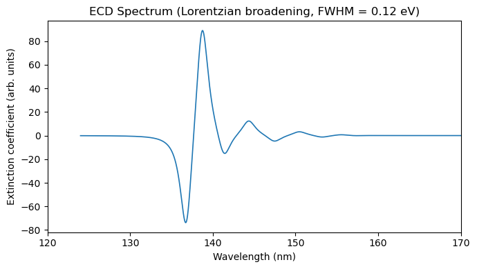
Text file
@jobs
task: exciton
@end

@method settings
xcfun: b3lyp
basis: cc-pvdz
@end

@exciton
fragments: 40
atoms_per_fragment: 55
nstates: 5
ct_nocc: 0
ct_nvir: 0
@end

@molecule
charge: 0
multiplicity: 1
xyz:
...
# XYZ coordinates for 40 x 55 atoms
...
@end- Norman, P., Ruud, K., & Saue, T. (2018). Principles and practices of molecular properties. John Wiley & Sons, Ltd.
- Jiemchooroj, A., & Norman, P. (2007). Electronic circular dichroism spectra from the complex polarization propagator. J. Chem. Phys., 126(13), 134102. 10.1063/1.2716660
- Norman, P., Ruud, K., & Helgaker, T. (2004). Density-functional theory calculations of optical rotatory dispersion in the nonresonant and resonant frequency regions. J. Chem. Phys., 120(11), 5027–5035. 10.1063/1.1647515
- Rosenfeld, L. (1929). Quantenmechanische Theorie der nat"urlichen optischen Aktivit"at von Fl"ussigkeiten und Gasen. Zeitschrift f"ur Physik, 52(3–4), 161–174. 10.1007/BF01342393
- Li, X., Parrish, R. M., Liu, F., Kokkila Schumacher, S. I. L., & Martinez, T. J. (2017). An Ab Initio Exciton Model Including Charge-Transfer Excited States. J. Chem. Theory Comput., 13(8), 3493–3504. 10.1021/acs.jctc.7b00171