VeloxChem provides access to a range of X‑ray spectroscopies by combining density‑functional theory with response theory techniques that enable the description of core‑level excitations and their characteristic spectral signatures. These methods allow the simulation of X‑ray absorption, emission, and related core‑level properties, thereby enabling chemically intuitive interpretation of spectral features. For a comprehensive review of theoretical approaches to X‑ray spectroscopies, see Norman & Dreuw (2018).
The ESCA molecule, ethyl trifluoroacetate (CF₃–CO–O–CH₂–CH₃), became historically important in X‑ray and photoelectron spectroscopies because its C 1s photoelectron spectrum displays four well‑separated and chemically distinct carbon binding energies, spanning more than 8 eV—a uniquely clear demonstration of chemical shifts arising from different charge environments at individual atomic sites. This spectrum rapidly became the pedagogical showcase for ESCA (Electron Spectroscopy for Chemical Analysis) following Kai Siegbahn’s development of high‑resolution photoelectron spectroscopy in the 1960s, and it has since served as a benchmark for both experimental methodology and theoretical modeling of core‑level shifts. The molecule continues to be used in modern X‑ray and photoelectron studies as a canonical reference system to illustrate how core‑level binding energies encode local electronic structure and substituent effects, linking directly to the foundational ESCA work recognized in Siegbahn’s 1981 Nobel Prize.
import veloxchem as vlx

molecule = vlx.Molecule.read_xyz_string("""13
b3lyp/def2-svp optimized geometry
C              1.326024532622         0.471089167011        -1.154937296389
C              0.484399509715         0.908494386259         0.037569541020
C              0.270494167717        -0.188493907246         1.053914467110
O              0.701245126416        -1.308212251798         0.971080711541
C             -0.582260522270         0.210893702941         2.291730106998
F             -0.731967860619        -0.799813015071         3.135965340271
F             -1.800383044157         0.625073687043         1.897202571864
F              0.003899498844         1.231896946553         2.943599980006
H              1.453639490166         1.302028888463        -1.864264306255
H              0.853135331881        -0.368249103011        -1.686230702784
H              2.322713498820         0.134038471332        -0.833394707486
H              0.936346512410         1.764030447212         0.571699332428
H             -0.514670521097         1.267150587304        -0.270103071648""")

molecule.show(atom_indices=True)XPS
X-ray Photoelectron Spectroscopy (XPS) probes the binding energies of core electrons and yields element-specific, chemically sensitive spectra in which each peak reflects the local electronic environment of an individual atomic site. In VeloxChem, XPS binding energies are obtained through the ΔSCF approach: a ground-state SCF calculation is performed first, followed by a separate unrestricted SCF calculation for each core-hole state (i.e., one core electron is removed from the targeted atom). The binding energy for each site is then computed as the difference in total energies between the core-ionized and ground states, along with a correction for relativistic and relaxation effects. The XPSDriver automates this workflow—it iterates over all atoms of the chosen element, generates the corresponding core-hole reference states, and assembles the final spectrum.
Python script
import veloxchem as vlx

molecule = vlx.Molecule.read_xyz_string("""13
ESCA b3lyp/def2-svp optimized geometry
C              1.326024532622         0.471089167011        -1.154937296389
C              0.484399509715         0.908494386259         0.037569541020
C              0.270494167717        -0.188493907246         1.053914467110
O              0.701245126416        -1.308212251798         0.971080711541
C             -0.582260522270         0.210893702941         2.291730106998
F             -0.731967860619        -0.799813015071         3.135965340271
F             -1.800383044157         0.625073687043         1.897202571864
F              0.003899498844         1.231896946553         2.943599980006
H              1.453639490166         1.302028888463        -1.864264306255
H              0.853135331881        -0.368249103011        -1.686230702784
H              2.322713498820         0.134038471332        -0.833394707486
H              0.936346512410         1.764030447212         0.571699332428
H             -0.514670521097         1.267150587304        -0.270103071648""")

basis = vlx.MolecularBasis.read(molecule, "def2-svp")

scf_drv = vlx.ScfRestrictedDriver()
scf_drv.xcfun = "b3lyp"
scf_results = scf_drv.compute(molecule, basis)

xps_drv = vlx.XPSDriver()

xps_results_c = xps_drv.compute(molecule, basis, scf_drv, element='C')
xps_drv.plot_spectrum(xps_results_c, element='C', broadening_type='lorentzian', broadening_value=1.0)
Self Consistent Field Driver Setup
====================================
Wave Function Model : Spin-Restricted Kohn-Sham
Initial Guess Model : Superposition of Atomic Densities
Convergence Accelerator : Two Level Direct Inversion of Iterative Subspace
Max. Number of Iterations : 50
Max. Number of Error Vectors : 10
Convergence Threshold : 1.0e-06
ERI Screening Threshold : 1.0e-12
Linear Dependence Threshold : 1.0e-06
Exchange-Correlation Functional : B3LYP
Molecular Grid Level : 4
* Info * Using the B3LYP functional.
P. J. Stephens, F. J. Devlin, C. F. Chabalowski, and M. J. Frisch., J. Phys. Chem. 98, 11623 (1994)
* Info * Using the Libxc library (v7.0.0).
S. Lehtola, C. Steigemann, M. J.T. Oliveira, and M. A.L. Marques., SoftwareX 7, 1–5 (2018)
* Info * Using the following algorithm for XC numerical integration.
J. Kussmann, H. Laqua and C. Ochsenfeld, J. Chem. Theory Comput. 2021, 17, 1512-1521
* Info * Starting Reduced Basis SCF calculation...
* Info * ...done. SCF energy in reduced basis set: -526.938455740283 a.u. Time: 0.95 sec.
Iter. | Kohn-Sham Energy | Energy Change | Gradient Norm | Max. Gradient | Density Change
--------------------------------------------------------------------------------------------
1 -529.744620047957 0.0000000000 0.68187132 0.04451920 0.00000000
2 -529.761724189171 -0.0171041412 0.52853611 0.02994243 0.34292965
3 -529.785309905891 -0.0235857167 0.18859233 0.01154555 0.18544344
4 -529.788269310006 -0.0029594041 0.05989831 0.00344551 0.07752242
5 -529.788585911978 -0.0003166020 0.00958419 0.00082579 0.02089948
6 -529.788594060748 -0.0000081488 0.00131577 0.00006847 0.00345142
7 -529.788594198377 -0.0000001376 0.00081039 0.00003744 0.00068283
8 -529.788594267176 -0.0000000688 0.00011457 0.00000605 0.00028403
9 -529.788594268230 -0.0000000011 0.00004229 0.00000202 0.00005041
10 -529.788594268395 -0.0000000002 0.00000776 0.00000045 0.00001442
11 -529.788594268402 -0.0000000000 0.00000252 0.00000012 0.00000351
12 -529.788594268402 -0.0000000000 0.00000059 0.00000003 0.00000128
*** SCF converged in 12 iterations. Time: 13.52 sec.
Spin-Restricted Kohn-Sham:
--------------------------
Total Energy : -529.7885942684 a.u.
Electronic Energy : -939.6986832343 a.u.
Nuclear Repulsion Energy : 409.9100889659 a.u.
------------------------------------
Gradient Norm : 0.0000005919 a.u.
Ground State Information
------------------------
Charge of Molecule : 0.0
Multiplicity (2S+1) : 1
Magnetic Quantum Number (M_S) : 0.0
XPS Driver
============
* Info * Computing core ionization energies for element(s): C
* Info * Method type: DFT
* Info * XC functional: B3LYP
* Info * Using DFT energy ranges for core orbital identification
* Info * Processing element: C
* Info * ------------------------------------------------------------
* Info * Found 4 core orbital(s) for C:
* Info * MO 4 -> Atom 5 (C) with 97.9% contribution
* Info * MO 5 -> Atom 3 (C) with 98.0% contribution
* Info * MO 6 -> Atom 2 (C) with 98.2% contribution
* Info * MO 7 -> Atom 1 (C) with 98.1% contribution
* Info * Computing FCH for C orbital 4 (Atom 5, contribution: 97.9%)...
Self Consistent Field Driver Setup
====================================
Wave Function Model : Spin-Unrestricted Kohn-Sham
Initial Guess Model : User Supplied Orbitals
Convergence Accelerator : Direct Inversion of Iterative Subspace
Max. Number of Iterations : 50
Max. Number of Error Vectors : 10
Convergence Threshold : 1.0e-06
ERI Screening Threshold : 1.0e-12
Linear Dependence Threshold : 1.0e-06
Exchange-Correlation Functional : B3LYP
Molecular Grid Level : 4
* Info * Using the B3LYP functional.
P. J. Stephens, F. J. Devlin, C. F. Chabalowski, and M. J. Frisch., J. Phys. Chem. 98, 11623 (1994)
* Info * Using the Libxc library (v7.0.0).
S. Lehtola, C. Steigemann, M. J.T. Oliveira, and M. A.L. Marques., SoftwareX 7, 1–5 (2018)
* Info * Using the following algorithm for XC numerical integration.
J. Kussmann, H. Laqua and C. Ochsenfeld, J. Chem. Theory Comput. 2021, 17, 1512-1521
* Info * Starting from user supplied orbitals
Iter. | Kohn-Sham Energy | Energy Change | Gradient Norm | Max. Gradient | Density Change
--------------------------------------------------------------------------------------------
1 -518.289010077889 0.0000000000 2.09106208 0.14588425 0.00000000
2 -516.742082018496 1.5469280594 4.31219465 0.21681912 2.40766509
3 -518.670776640964 -1.9286946225 0.88329431 0.05562338 1.79151673
4 -518.697847191240 -0.0270705503 0.74102319 0.04892962 0.44847577
5 -518.747307831937 -0.0494606407 0.15826985 0.00941357 0.23791115
6 -518.750188913996 -0.0028810821 0.03645947 0.00156008 0.05865136
7 -518.750300118318 -0.0001112043 0.01581178 0.00084293 0.01358365
8 -518.750323586558 -0.0000234682 0.00469606 0.00023963 0.00533234
9 -518.750327323421 -0.0000037369 0.00223713 0.00016303 0.00262359
10 -518.750328270266 -0.0000009468 0.00069048 0.00004129 0.00145704
11 -518.750328365306 -0.0000000950 0.00016832 0.00000853 0.00053424
12 -518.750328368438 -0.0000000031 0.00014040 0.00000616 0.00011174
13 -518.750328370856 -0.0000000024 0.00003983 0.00000251 0.00005266
14 -518.750328371270 -0.0000000004 0.00002553 0.00000194 0.00002181
15 -518.750328371603 -0.0000000003 0.00001511 0.00000158 0.00002547
16 -518.750328371702 -0.0000000001 0.00000616 0.00000047 0.00001652
17 -518.750328371717 -0.0000000000 0.00000229 0.00000013 0.00000694
18 -518.750328371718 -0.0000000000 0.00000113 0.00000006 0.00000181
19 -518.750328371718 0.0000000000 0.00000112 0.00000006 0.00000070
20 -518.750328371718 0.0000000000 0.00000026 0.00000001 0.00000045
*** SCF converged in 20 iterations. Time: 43.27 sec.
Spin-Unrestricted Kohn-Sham:
----------------------------
Total Energy : -518.7503283717 a.u.
Electronic Energy : -928.6604173376 a.u.
Nuclear Repulsion Energy : 409.9100889659 a.u.
------------------------------------
Gradient Norm : 0.0000002564 a.u.
Ground State Information
------------------------
Charge of Molecule : 1.0
Multiplicity (2S+1) : 2
Magnetic Quantum Number (M_S) : 0.5
Expectation value of S**2 : 0.7586
* Info * Orbital 4 (Atom 5): Ionization Energy = 300.37 eV
* Info * Computing FCH for C orbital 5 (Atom 3, contribution: 98.0%)...
Self Consistent Field Driver Setup
====================================
Wave Function Model : Spin-Unrestricted Kohn-Sham
Initial Guess Model : User Supplied Orbitals
Convergence Accelerator : Direct Inversion of Iterative Subspace
Max. Number of Iterations : 50
Max. Number of Error Vectors : 10
Convergence Threshold : 1.0e-06
ERI Screening Threshold : 1.0e-12
Linear Dependence Threshold : 1.0e-06
Exchange-Correlation Functional : B3LYP
Molecular Grid Level : 4
* Info * Using the B3LYP functional.
P. J. Stephens, F. J. Devlin, C. F. Chabalowski, and M. J. Frisch., J. Phys. Chem. 98, 11623 (1994)
* Info * Using the Libxc library (v7.0.0).
S. Lehtola, C. Steigemann, M. J.T. Oliveira, and M. A.L. Marques., SoftwareX 7, 1–5 (2018)
* Info * Using the following algorithm for XC numerical integration.
J. Kussmann, H. Laqua and C. Ochsenfeld, J. Chem. Theory Comput. 2021, 17, 1512-1521
* Info * Starting from user supplied orbitals
Iter. | Kohn-Sham Energy | Energy Change | Gradient Norm | Max. Gradient | Density Change
--------------------------------------------------------------------------------------------
1 -518.422092868206 0.0000000000 2.07204001 0.11573997 0.00000000
2 -517.685701575948 0.7363912923 3.14009819 0.15939317 2.13078623
3 -518.830437846163 -1.1447362702 0.78398928 0.05282656 1.42962840
4 -518.868867144228 -0.0384292981 0.42586853 0.02291159 0.33018199
5 -518.887704953591 -0.0188378094 0.15033422 0.00843206 0.19474989
6 -518.889999291205 -0.0022943376 0.03199004 0.00182300 0.05129826
7 -518.890131562353 -0.0001322711 0.01189504 0.00081198 0.01358688
8 -518.890171610252 -0.0000400479 0.00611816 0.00058654 0.00611461
9 -518.890205196091 -0.0000335858 0.00406637 0.00032522 0.00793256
10 -518.890221623691 -0.0000164276 0.00187940 0.00017296 0.00727382
11 -518.890224009679 -0.0000023860 0.00117062 0.00006149 0.00304259
12 -518.890224384027 -0.0000003743 0.00038982 0.00002107 0.00108387
13 -518.890224431153 -0.0000000471 0.00007854 0.00000652 0.00041277
14 -518.890224434698 -0.0000000035 0.00003956 0.00000253 0.00012541
15 -518.890224435050 -0.0000000004 0.00002108 0.00000129 0.00004027
16 -518.890224435100 -0.0000000001 0.00001472 0.00000111 0.00001489
17 -518.890224435116 -0.0000000000 0.00000876 0.00000053 0.00000831
18 -518.890224435124 -0.0000000000 0.00000125 0.00000006 0.00000281
19 -518.890224435125 -0.0000000000 0.00000073 0.00000003 0.00000089
*** SCF converged in 19 iterations. Time: 40.36 sec.
Spin-Unrestricted Kohn-Sham:
----------------------------
Total Energy : -518.8902244351 a.u.
Electronic Energy : -928.8003134010 a.u.
Nuclear Repulsion Energy : 409.9100889659 a.u.
------------------------------------
Gradient Norm : 0.0000007349 a.u.
Ground State Information
------------------------
Charge of Molecule : 1.0
Multiplicity (2S+1) : 2
Magnetic Quantum Number (M_S) : 0.5
Expectation value of S**2 : 0.7713
* Info * Orbital 5 (Atom 3): Ionization Energy = 296.56 eV
* Info * Computing FCH for C orbital 6 (Atom 2, contribution: 98.2%)...
Self Consistent Field Driver Setup
====================================
Wave Function Model : Spin-Unrestricted Kohn-Sham
Initial Guess Model : User Supplied Orbitals
Convergence Accelerator : Direct Inversion of Iterative Subspace
Max. Number of Iterations : 50
Max. Number of Error Vectors : 10
Convergence Threshold : 1.0e-06
ERI Screening Threshold : 1.0e-12
Linear Dependence Threshold : 1.0e-06
Exchange-Correlation Functional : B3LYP
Molecular Grid Level : 4
* Info * Using the B3LYP functional.
P. J. Stephens, F. J. Devlin, C. F. Chabalowski, and M. J. Frisch., J. Phys. Chem. 98, 11623 (1994)
* Info * Using the Libxc library (v7.0.0).
S. Lehtola, C. Steigemann, M. J.T. Oliveira, and M. A.L. Marques., SoftwareX 7, 1–5 (2018)
* Info * Using the following algorithm for XC numerical integration.
J. Kussmann, H. Laqua and C. Ochsenfeld, J. Chem. Theory Comput. 2021, 17, 1512-1521
* Info * Starting from user supplied orbitals
Iter. | Kohn-Sham Energy | Energy Change | Gradient Norm | Max. Gradient | Density Change
--------------------------------------------------------------------------------------------
1 -518.508884323095 0.0000000000 2.11041577 0.15986426 0.00000000
2 -518.061074626334 0.4478096968 2.78705243 0.13663979 2.22449185
3 -518.917328433711 -0.8562538074 0.88812839 0.06038146 1.42355403
4 -518.977597351797 -0.0602689181 0.40727618 0.02597099 0.36586234
5 -518.993403617599 -0.0158062658 0.03857147 0.00190002 0.13221775
6 -518.993555058096 -0.0001514405 0.01408871 0.00084794 0.01748692
7 -518.993573969597 -0.0000189115 0.00707527 0.00054063 0.00550138
8 -518.993579233889 -0.0000052643 0.00186508 0.00012807 0.00261067
9 -518.993580103139 -0.0000008693 0.00074964 0.00004055 0.00142002
10 -518.993580232445 -0.0000001293 0.00024990 0.00001530 0.00056816
11 -518.993580243908 -0.0000000115 0.00007691 0.00000797 0.00014676
12 -518.993580247306 -0.0000000034 0.00004263 0.00000376 0.00007527
13 -518.993580248349 -0.0000000010 0.00003503 0.00000196 0.00003953
14 -518.993580248884 -0.0000000005 0.00001352 0.00000075 0.00003544
15 -518.993580248950 -0.0000000001 0.00000837 0.00000050 0.00001449
16 -518.993580248962 -0.0000000000 0.00000227 0.00000014 0.00000536
17 -518.993580248963 -0.0000000000 0.00000103 0.00000006 0.00000177
18 -518.993580248963 0.0000000000 0.00000034 0.00000002 0.00000055
*** SCF converged in 18 iterations. Time: 38.27 sec.
Spin-Unrestricted Kohn-Sham:
----------------------------
Total Energy : -518.9935802490 a.u.
Electronic Energy : -928.9036692149 a.u.
Nuclear Repulsion Energy : 409.9100889659 a.u.
------------------------------------
Gradient Norm : 0.0000003373 a.u.
Ground State Information
------------------------
Charge of Molecule : 1.0
Multiplicity (2S+1) : 2
Magnetic Quantum Number (M_S) : 0.5
Expectation value of S**2 : 0.7573
* Info * Orbital 6 (Atom 2): Ionization Energy = 293.75 eV
* Info * Computing FCH for C orbital 7 (Atom 1, contribution: 98.1%)...
Self Consistent Field Driver Setup
====================================
Wave Function Model : Spin-Unrestricted Kohn-Sham
Initial Guess Model : User Supplied Orbitals
Convergence Accelerator : Direct Inversion of Iterative Subspace
Max. Number of Iterations : 50
Max. Number of Error Vectors : 10
Convergence Threshold : 1.0e-06
ERI Screening Threshold : 1.0e-12
Linear Dependence Threshold : 1.0e-06
Exchange-Correlation Functional : B3LYP
Molecular Grid Level : 4
* Info * Using the B3LYP functional.
P. J. Stephens, F. J. Devlin, C. F. Chabalowski, and M. J. Frisch., J. Phys. Chem. 98, 11623 (1994)
* Info * Using the Libxc library (v7.0.0).
S. Lehtola, C. Steigemann, M. J.T. Oliveira, and M. A.L. Marques., SoftwareX 7, 1–5 (2018)
* Info * Using the following algorithm for XC numerical integration.
J. Kussmann, H. Laqua and C. Ochsenfeld, J. Chem. Theory Comput. 2021, 17, 1512-1521
* Info * Starting from user supplied orbitals
Iter. | Kohn-Sham Energy | Energy Change | Gradient Norm | Max. Gradient | Density Change
--------------------------------------------------------------------------------------------
1 -518.530549082057 0.0000000000 2.08989144 0.23728857 0.00000000
2 -518.367398472093 0.1631506100 2.25537758 0.13624142 1.95101635
3 -519.003745824938 -0.6363473528 0.18375578 0.00909997 1.17605497
4 -519.005663342683 -0.0019175177 0.13953631 0.00914748 0.11878336
5 -519.007299643134 -0.0016363005 0.04715966 0.00319590 0.06696039
6 -519.007522514420 -0.0002228713 0.01137274 0.00049793 0.01669728
7 -519.007537115496 -0.0000146011 0.00553061 0.00038337 0.00467953
8 -519.007541467759 -0.0000043523 0.00171304 0.00011455 0.00257847
9 -519.007542060828 -0.0000005931 0.00068050 0.00003220 0.00120364
10 -519.007542133996 -0.0000000732 0.00028291 0.00001363 0.00045337
11 -519.007542141502 -0.0000000075 0.00006416 0.00000333 0.00011155
12 -519.007542141860 -0.0000000004 0.00002293 0.00000122 0.00002627
13 -519.007542141933 -0.0000000001 0.00000606 0.00000050 0.00001168
14 -519.007542141944 -0.0000000000 0.00000346 0.00000022 0.00000470
15 -519.007542141948 -0.0000000000 0.00000187 0.00000014 0.00000241
16 -519.007542141949 -0.0000000000 0.00000127 0.00000013 0.00000161
17 -519.007542141950 -0.0000000000 0.00000064 0.00000007 0.00000097
*** SCF converged in 17 iterations. Time: 35.63 sec.
Spin-Unrestricted Kohn-Sham:
----------------------------
Total Energy : -519.0075421419 a.u.
Electronic Energy : -928.9176311078 a.u.
Nuclear Repulsion Energy : 409.9100889659 a.u.
------------------------------------
Gradient Norm : 0.0000006391 a.u.
Ground State Information
------------------------
Charge of Molecule : 1.0
Multiplicity (2S+1) : 2
Magnetic Quantum Number (M_S) : 0.5
Expectation value of S**2 : 0.7571
* Info * Orbital 7 (Atom 1): Ionization Energy = 293.37 eV
*** XPS Calculation Completed.
xps_drv.plot_spectrum(xps_results_c, element='C', broadening_type='lorentzian', broadening_value=1.0)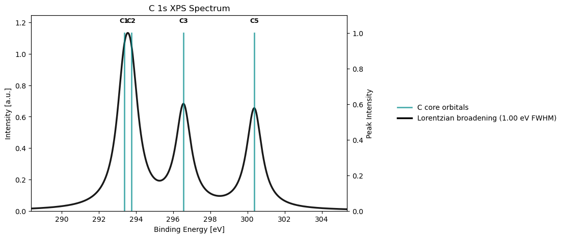
XPS spectra can also be calculated for several elements at a time:
# Compute XPS for C, O, and F at once
xps_multi = xps_drv.compute(molecule, basis, scf_drv, element=['C', 'O', 'F'])

# Plot 1: Carbon with atom labels (default)
xps_drv.plot_spectrum(xps_multi, element='C', color='vlx',
                      broadening_value=1.0, show_atom_labels=True)
# Plot 2: Carbon color-coded by atom
xps_drv.plot_spectrum(xps_multi, element='C', color='cpk',
                      broadening_value=1.0, color_by_atom=True)

# Plot 3: Oxygen with atom labels
xps_drv.plot_spectrum(xps_multi, element='O', color='cpk',
                      broadening_value=1.0)

# Plot 4: Fluorine with atom labels
xps_drv.plot_spectrum(xps_multi, element='F', color='cpk',
broadening_value=1.0)Text file
@jobs
task: xps
@end

@method settings
xcfun: b3lyp
basis: def2-svp
@end

@xps
element: C, O
@end

@molecule
charge: 0
multiplicity: 1
xyz:
...
@end
XAS
X-ray absorption spectra in the near-edge region, often referred to as NEXAFS or XANES, can be calculated in VeloxChem in two complementary ways. The CVS approach, based on the linear-response eigensolver with core-valence separation, targets discrete core-excited states for a selected edge. The CPP solver instead samples the absorption response over a chosen frequency window and is convenient when you want a continuous spectrum directly. In terms of choice of functional, the version of the CAM-B3LYP functional with 100% exchange in the asymptotic limit as introduced by Ekström & Norman (2006) has been shown in a comprehensive benchmark study to perform particularly well, see Fransson et al. (2021).
XAS with CVS
In the CVS formulation, the excitation space is restricted to core-to-virtual transitions. This makes it straightforward to target a specific edge by selecting how many core orbitals should be included.
Python script
import veloxchem as vlx

molecule = vlx.Molecule.read_xyz_string("""13
ESCA b3lyp/def2-svp optimized geometry
C              1.326024532622         0.471089167011        -1.154937296389
C              0.484399509715         0.908494386259         0.037569541020
C              0.270494167717        -0.188493907246         1.053914467110
O              0.701245126416        -1.308212251798         0.971080711541
C             -0.582260522270         0.210893702941         2.291730106998
F             -0.731967860619        -0.799813015071         3.135965340271
F             -1.800383044157         0.625073687043         1.897202571864
F              0.003899498844         1.231896946553         2.943599980006
H              1.453639490166         1.302028888463        -1.864264306255
H              0.853135331881        -0.368249103011        -1.686230702784
H              2.322713498820         0.134038471332        -0.833394707486
H              0.936346512410         1.764030447212         0.571699332428
H             -0.514670521097         1.267150587304        -0.270103071648""")

basis = vlx.MolecularBasis.read(molecule, "def2-svp")

scf_drv = vlx.ScfRestrictedDriver()
scf_drv.xcfun = "cam-b3lyp-100"
scf_results = scf_drv.compute(molecule, basis)

rsp_drv = vlx.LinearResponseEigenSolver()
rsp_drv.core_excitation = True

# Include all occupied orbitals up to and including the C 1s manifold
rsp_drv.num_core_orbitals = 8
rsp_drv.nstates = 20

rsp_results = rsp_drv.compute(molecule, basis, scf_results)
rsp_drv.plot_xas(rsp_results)
Self Consistent Field Driver Setup
====================================
Wave Function Model : Spin-Restricted Kohn-Sham
Initial Guess Model : Superposition of Atomic Densities
Convergence Accelerator : Two Level Direct Inversion of Iterative Subspace
Max. Number of Iterations : 50
Max. Number of Error Vectors : 10
Convergence Threshold : 1.0e-06
ERI Screening Threshold : 1.0e-12
Linear Dependence Threshold : 1.0e-06
Exchange-Correlation Functional : CAM-B3LYP-100
Molecular Grid Level : 4
* Info * Using the CAM-B3LYP-100 functional.
T. Yanai, D. P. Tew, and N. C. Handy., Chem. Phys. Lett. 393, 51 (2004)
* Info * Using the Libxc library (v7.0.0).
S. Lehtola, C. Steigemann, M. J.T. Oliveira, and M. A.L. Marques., SoftwareX 7, 1–5 (2018)
* Info * Using the following algorithm for XC numerical integration.
J. Kussmann, H. Laqua and C. Ochsenfeld, J. Chem. Theory Comput. 2021, 17, 1512-1521
* Info * Starting Reduced Basis SCF calculation...
* Info * ...done. SCF energy in reduced basis set: -526.938455740283 a.u. Time: 0.86 sec.
Iter. | Kohn-Sham Energy | Energy Change | Gradient Norm | Max. Gradient | Density Change
--------------------------------------------------------------------------------------------
1 -529.288350879602 0.0000000000 0.45365976 0.03048667 0.00000000
2 -529.302484244394 -0.0141333648 0.26812872 0.01557352 0.20251141
3 -529.308171569532 -0.0056873251 0.08402145 0.00450568 0.08899941
4 -529.308755189458 -0.0005836199 0.01926955 0.00116110 0.02427703
5 -529.308788399387 -0.0000332099 0.00773721 0.00052732 0.00993577
6 -529.308794747364 -0.0000063480 0.00131958 0.00006227 0.00310100
7 -529.308795126858 -0.0000003795 0.00029120 0.00001198 0.00140409
8 -529.308795145506 -0.0000000186 0.00015140 0.00000705 0.00028925
9 -529.308795148616 -0.0000000031 0.00004070 0.00000191 0.00009471
10 -529.308795148847 -0.0000000002 0.00001744 0.00000069 0.00002906
11 -529.308795148893 -0.0000000000 0.00000365 0.00000017 0.00001149
12 -529.308795148895 -0.0000000000 0.00000065 0.00000003 0.00000377
*** SCF converged in 12 iterations. Time: 19.36 sec.
Spin-Restricted Kohn-Sham:
--------------------------
Total Energy : -529.3087951489 a.u.
Electronic Energy : -939.2188841148 a.u.
Nuclear Repulsion Energy : 409.9100889659 a.u.
------------------------------------
Gradient Norm : 0.0000006493 a.u.
Ground State Information
------------------------
Charge of Molecule : 0.0
Multiplicity (2S+1) : 1
Magnetic Quantum Number (M_S) : 0.0
Linear Response EigenSolver Setup
===================================
Number of States : 20
Max. Number of Iterations : 150
Convergence Threshold : 1.0e-04
ERI Screening Threshold : 1.0e-12
Exchange-Correlation Functional : CAM-B3LYP-100
Molecular Grid Level : 4
* Info * Using the CAM-B3LYP-100 functional.
T. Yanai, D. P. Tew, and N. C. Handy., Chem. Phys. Lett. 393, 51 (2004)
* Info * Using the Libxc library (v7.0.0).
S. Lehtola, C. Steigemann, M. J.T. Oliveira, and M. A.L. Marques., SoftwareX 7, 1–5 (2018)
* Info * Using the following algorithm for XC numerical integration.
J. Kussmann, H. Laqua and C. Ochsenfeld, J. Chem. Theory Comput. 2021, 17, 1512-1521
* Info * 40 gerade trial vectors in reduced space
* Info * 40 ungerade trial vectors in reduced space
*** Iteration: 1 * Residuals (Max,Min): 1.43e-01 and 4.38e-02
* Info * 60 gerade trial vectors in reduced space
* Info * 60 ungerade trial vectors in reduced space
*** Iteration: 2 * Residuals (Max,Min): 5.50e-02 and 4.87e-03
* Info * 80 gerade trial vectors in reduced space
* Info * 80 ungerade trial vectors in reduced space
*** Iteration: 3 * Residuals (Max,Min): 1.32e-02 and 8.67e-04
* Info * 100 gerade trial vectors in reduced space
* Info * 100 ungerade trial vectors in reduced space
*** Iteration: 4 * Residuals (Max,Min): 5.98e-03 and 6.88e-05
* Info * 119 gerade trial vectors in reduced space
* Info * 119 ungerade trial vectors in reduced space
*** Iteration: 5 * Residuals (Max,Min): 2.31e-03 and 5.09e-06
* Info * 124 gerade trial vectors in reduced space
* Info * 124 ungerade trial vectors in reduced space
*** Iteration: 6 * Residuals (Max,Min): 6.12e-04 and 5.08e-06
* Info * 125 gerade trial vectors in reduced space
* Info * 126 ungerade trial vectors in reduced space
*** Iteration: 7 * Residuals (Max,Min): 1.48e-04 and 5.08e-06
* Info * 126 gerade trial vectors in reduced space
* Info * 127 ungerade trial vectors in reduced space
*** Iteration: 8 * Residuals (Max,Min): 9.62e-05 and 5.08e-06
*** Linear response converged in 8 iterations. Time: 178.91 sec
Electric Transition Dipole Moments (dipole length, a.u.)
--------------------------------------------------------
X Y Z
Excited State S1: -0.077516 -0.026497 -0.044904
Excited State S2: 0.000545 0.000183 0.000321
Excited State S3: -0.001499 -0.000520 -0.000902
Excited State S4: 0.014317 0.002784 -0.026347
Excited State S5: -0.018791 0.039380 0.009137
Excited State S6: 0.007741 -0.061489 0.022414
Excited State S7: 0.053143 0.017919 0.030878
Excited State S8: 0.060495 0.020789 0.035034
Excited State S9: 0.013499 -0.016837 -0.013342
Excited State S10: -0.010067 -0.026255 0.033099
Excited State S11: -0.033211 0.010881 0.050943
Excited State S12: -0.018021 -0.006189 -0.010348
Excited State S13: -0.003322 0.031720 -0.013073
Excited State S14: 0.016517 -0.013254 -0.020721
Excited State S15: 0.035907 0.012243 0.020735
Excited State S16: 0.006082 -0.010979 -0.003939
Excited State S17: -0.013036 -0.004699 -0.007027
Excited State S18: 0.011185 0.025806 -0.035009
Excited State S19: 0.010358 -0.016954 -0.007787
Excited State S20: -0.010788 0.025400 0.003756
Electric Transition Dipole Moments (dipole velocity, a.u.)
----------------------------------------------------------
X Y Z
Excited State S1: -0.076381 -0.026107 -0.044245
Excited State S2: 0.001406 0.000479 0.000820
Excited State S3: -0.001608 -0.000557 -0.000964
Excited State S4: 0.014560 0.002434 -0.026562
Excited State S5: -0.019157 0.040520 0.009093
Excited State S6: 0.008359 -0.062911 0.022176
Excited State S7: 0.054330 0.018319 0.031564
Excited State S8: 0.061540 0.021150 0.035647
Excited State S9: 0.011416 -0.015584 -0.010492
Excited State S10: -0.008226 -0.027648 0.030751
Excited State S11: -0.032959 0.010750 0.050587
Excited State S12: -0.018325 -0.006295 -0.010527
Excited State S13: -0.003138 0.030563 -0.012704
Excited State S14: 0.016854 -0.013949 -0.020893
Excited State S15: 0.035739 0.012186 0.020637
Excited State S16: 0.006198 -0.012354 -0.003331
Excited State S17: -0.013211 -0.004731 -0.007126
Excited State S18: 0.011642 0.023840 -0.034644
Excited State S19: 0.010769 -0.017200 -0.008347
Excited State S20: -0.010268 0.023321 0.004078
Magnetic Transition Dipole Moments (a.u.)
-----------------------------------------
X Y Z
Excited State S1: 0.345626 -0.657300 -0.208806
Excited State S2: -0.013389 0.019988 0.011385
Excited State S3: -0.010780 0.030327 0.000472
Excited State S4: -0.089892 0.179086 -0.032862
Excited State S5: 0.063210 -0.050210 0.356940
Excited State S6: -0.604725 -0.378981 -0.847492
Excited State S7: 0.351621 -1.041345 -0.000565
Excited State S8: 0.307963 -0.168356 -0.431836
Excited State S9: -0.226897 0.005772 -0.255461
Excited State S10: 0.279029 -0.148954 -0.059288
Excited State S11: 0.353718 -0.282704 0.290535
Excited State S12: -0.119484 0.342168 0.003376
Excited State S13: -0.121625 0.059693 0.173646
Excited State S14: -0.183940 0.103983 -0.217811
Excited State S15: -0.230748 0.919022 -0.143061
Excited State S16: 0.132304 0.072337 -0.021983
Excited State S17: -0.061207 0.028622 0.094434
Excited State S18: -0.316020 0.168924 0.010047
Excited State S19: -0.233776 -0.013469 -0.273853
Excited State S20: -0.251139 -0.117891 0.041757
One-Photon Absorption
---------------------
Excited State S1: 10.13581699 a.u. 275.80963 eV Osc.Str. 0.0590
Excited State S2: 10.13742380 a.u. 275.85335 eV Osc.Str. 0.0000
Excited State S3: 10.17865089 a.u. 276.97520 eV Osc.Str. 0.0000
Excited State S4: 10.22246787 a.u. 278.16752 eV Osc.Str. 0.0062
Excited State S5: 10.23345984 a.u. 278.46663 eV Osc.Str. 0.0136
Excited State S6: 10.25215633 a.u. 278.97539 eV Osc.Str. 0.0297
Excited State S7: 10.25512063 a.u. 279.05605 eV Osc.Str. 0.0280
Excited State S8: 10.26407904 a.u. 279.29982 eV Osc.Str. 0.0364
Excited State S9: 10.29271531 a.u. 280.07905 eV Osc.Str. 0.0044
Excited State S10: 10.29805359 a.u. 280.22431 eV Osc.Str. 0.0129
Excited State S11: 10.31704474 a.u. 280.74109 eV Osc.Str. 0.0263
Excited State S12: 10.32494599 a.u. 280.95609 eV Osc.Str. 0.0032
Excited State S13: 10.33098443 a.u. 281.12041 eV Osc.Str. 0.0082
Excited State S14: 10.34973341 a.u. 281.63059 eV Osc.Str. 0.0061
Excited State S15: 10.35332123 a.u. 281.72822 eV Osc.Str. 0.0129
Excited State S16: 10.35736112 a.u. 281.83815 eV Osc.Str. 0.0012
Excited State S17: 10.36031045 a.u. 281.91841 eV Osc.Str. 0.0017
Excited State S18: 10.36345167 a.u. 282.00389 eV Osc.Str. 0.0139
Excited State S19: 10.39409773 a.u. 282.83781 eV Osc.Str. 0.0032
Excited State S20: 10.39961969 a.u. 282.98807 eV Osc.Str. 0.0054
Electronic Circular Dichroism
-----------------------------
Excited State S1: Rot.Str. -0.000000 a.u. -0.0001 [10**(-40) cgs]
Excited State S2: Rot.Str. 0.000000 a.u. 0.0000 [10**(-40) cgs]
Excited State S3: Rot.Str. -0.000000 a.u. -0.0000 [10**(-40) cgs]
Excited State S4: Rot.Str. -0.000000 a.u. -0.0000 [10**(-40) cgs]
Excited State S5: Rot.Str. 0.000000 a.u. 0.0001 [10**(-40) cgs]
Excited State S6: Rot.Str. -0.000007 a.u. -0.0034 [10**(-40) cgs]
Excited State S7: Rot.Str. 0.000010 a.u. 0.0045 [10**(-40) cgs]
Excited State S8: Rot.Str. -0.000002 a.u. -0.0011 [10**(-40) cgs]
Excited State S9: Rot.Str. 0.000000 a.u. 0.0001 [10**(-40) cgs]
Excited State S10: Rot.Str. -0.000000 a.u. -0.0000 [10**(-40) cgs]
Excited State S11: Rot.Str. 0.000000 a.u. 0.0000 [10**(-40) cgs]
Excited State S12: Rot.Str. 0.000000 a.u. 0.0001 [10**(-40) cgs]
Excited State S13: Rot.Str. -0.000000 a.u. -0.0000 [10**(-40) cgs]
Excited State S14: Rot.Str. 0.000000 a.u. 0.0001 [10**(-40) cgs]
Excited State S15: Rot.Str. 0.000000 a.u. 0.0001 [10**(-40) cgs]
Excited State S16: Rot.Str. -0.000000 a.u. -0.0002 [10**(-40) cgs]
Excited State S17: Rot.Str. 0.000000 a.u. 0.0001 [10**(-40) cgs]
Excited State S18: Rot.Str. -0.000000 a.u. -0.0000 [10**(-40) cgs]
Excited State S19: Rot.Str. -0.000000 a.u. -0.0000 [10**(-40) cgs]
Excited State S20: Rot.Str. -0.000000 a.u. -0.0001 [10**(-40) cgs]
Character of excitations:
Excited state 1
---------------
core_6 -> LUMO 0.9904
Excited state 2
---------------
core_7 -> LUMO -0.9938
Excited state 3
---------------
core_8 -> LUMO -0.9959
Excited state 4
---------------
core_8 -> LUMO+1 -0.9348
core_8 -> LUMO+2 -0.2589
Excited state 5
---------------
core_7 -> LUMO+1 -0.9254
core_7 -> LUMO+2 0.3002
Excited state 6
---------------
core_8 -> LUMO+4 -0.9007
core_8 -> LUMO+2 -0.3993
Excited state 7
---------------
core_8 -> LUMO+3 0.7429
core_8 -> LUMO+5 -0.6498
Excited state 8
---------------
core_7 -> LUMO+3 0.9442
core_7 -> LUMO+5 0.2619
Excited state 9
---------------
core_8 -> LUMO+2 0.8185
core_8 -> LUMO+4 -0.3635
core_8 -> LUMO+10 -0.3059
core_8 -> LUMO+1 -0.2059
Excited state 10
----------------
core_7 -> LUMO+2 -0.8152
core_7 -> LUMO+8 -0.3477
core_7 -> LUMO+6 -0.2721
core_7 -> LUMO+10 0.2296
core_7 -> LUMO+1 -0.2155
Excited state 11
----------------
core_8 -> LUMO+6 -0.6652
core_8 -> LUMO+10 0.4686
core_8 -> LUMO+7 -0.3399
core_8 -> LUMO+1 -0.2738
core_8 -> LUMO+2 0.2666
Excited state 12
----------------
core_8 -> LUMO+5 0.7314
core_8 -> LUMO+3 0.6565
Excited state 13
----------------
core_7 -> LUMO+4 0.7821
core_7 -> LUMO+6 -0.4344
core_7 -> LUMO+7 -0.2838
core_7 -> LUMO+8 0.2636
Excited state 14
----------------
core_7 -> LUMO+6 0.6856
core_7 -> LUMO+4 0.4397
core_7 -> LUMO+2 -0.3155
core_7 -> LUMO+10 -0.2767
core_7 -> LUMO+1 -0.2734
core_7 -> LUMO+7 0.2302
Excited state 15
----------------
core_5 -> LUMO -0.9730
Excited state 16
----------------
core_6 -> LUMO+1 0.8455
core_6 -> LUMO+6 0.4904
Excited state 17
----------------
core_7 -> LUMO+5 -0.9551
core_7 -> LUMO+3 0.2734
Excited state 18
----------------
core_7 -> LUMO+8 0.6697
core_7 -> LUMO+4 -0.4096
core_7 -> LUMO+2 -0.3494
core_7 -> LUMO+7 -0.3344
core_7 -> LUMO+10 -0.2583
core_7 -> LUMO+11 0.2145
Excited state 19
----------------
core_8 -> LUMO+8 0.8037
core_8 -> LUMO+7 -0.4535
core_8 -> LUMO+10 -0.2051
core_8 -> LUMO+11 0.2050
core_8 -> LUMO+12 -0.2026
Excited state 20
----------------
core_6 -> LUMO+6 -0.7081
core_6 -> LUMO+2 -0.4443
core_6 -> LUMO+1 0.3319
core_6 -> LUMO+4 0.3292
rsp_drv.plot_xas(rsp_results)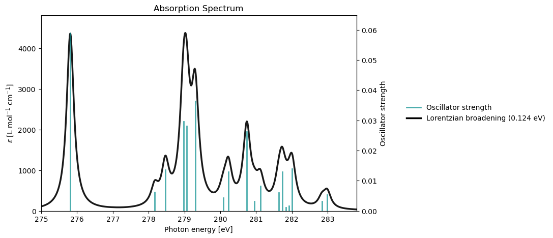
Text file
@jobs
task: response
@end

@method settings
xcfun: cam-b3lyp
basis: def2-svp
@end

@response
property: absorption
core_excitation: yes
num_core_orbitals: 8
nstates: 20
@end

@molecule
charge: 0
multiplicity: 1
xyz:
...
@end
For the CVS calculation, num_core_orbitals is the number of occupied core orbitals included up to the edge of interest when the occupied orbitals are ordered by energy. For ESCA, 8 corresponds to the three F 1s orbitals, one O 1s orbital, and four C 1s orbitals, so it reaches and includes the full C 1s manifold.
XAS with CPP
In the CPP formulation, the absorption cross section is evaluated directly over a user-defined frequency window. This is useful when you want the near-edge spectral profile without solving explicitly for individual excited states.
Python script
import veloxchem as vlx
import numpy as np

molecule = vlx.Molecule.read_xyz_string("""13
ESCA b3lyp/def2-svp optimized geometry
C              1.326024532622         0.471089167011        -1.154937296389
C              0.484399509715         0.908494386259         0.037569541020
C              0.270494167717        -0.188493907246         1.053914467110
O              0.701245126416        -1.308212251798         0.971080711541
C             -0.582260522270         0.210893702941         2.291730106998
F             -0.731967860619        -0.799813015071         3.135965340271
F             -1.800383044157         0.625073687043         1.897202571864
F              0.003899498844         1.231896946553         2.943599980006
H              1.453639490166         1.302028888463        -1.864264306255
H              0.853135331881        -0.368249103011        -1.686230702784
H              2.322713498820         0.134038471332        -0.833394707486
H              0.936346512410         1.764030447212         0.571699332428
H             -0.514670521097         1.267150587304        -0.270103071648""")

basis = vlx.MolecularBasis.read(molecule, "def2-svp")

scf_drv = vlx.ScfRestrictedDriver()
scf_drv.xcfun = "cam-b3lyp-100"
scf_results = scf_drv.compute(molecule, basis)

cpp_drv = vlx.ComplexResponse()
cpp_drv.frequencies = np.arange(10.1, 10.4, 0.0025)
cpp_drv.property = "absorption"

cpp_results = cpp_drv.compute(molecule, basis, scf_results)
cpp_drv.plot(cpp_results, x_unit="eV")
Self Consistent Field Driver Setup
====================================
Wave Function Model : Spin-Restricted Kohn-Sham
Initial Guess Model : Superposition of Atomic Densities
Convergence Accelerator : Two Level Direct Inversion of Iterative Subspace
Max. Number of Iterations : 50
Max. Number of Error Vectors : 10
Convergence Threshold : 1.0e-06
ERI Screening Threshold : 1.0e-12
Linear Dependence Threshold : 1.0e-06
Exchange-Correlation Functional : CAM-B3LYP-100
Molecular Grid Level : 4
* Info * Using the CAM-B3LYP-100 functional.
T. Yanai, D. P. Tew, and N. C. Handy., Chem. Phys. Lett. 393, 51 (2004)
* Info * Using the Libxc library (v7.0.0).
S. Lehtola, C. Steigemann, M. J.T. Oliveira, and M. A.L. Marques., SoftwareX 7, 1–5 (2018)
* Info * Using the following algorithm for XC numerical integration.
J. Kussmann, H. Laqua and C. Ochsenfeld, J. Chem. Theory Comput. 2021, 17, 1512-1521
* Info * Starting Reduced Basis SCF calculation...
* Info * ...done. SCF energy in reduced basis set: -526.938455740282 a.u. Time: 0.88 sec.
Iter. | Kohn-Sham Energy | Energy Change | Gradient Norm | Max. Gradient | Density Change
--------------------------------------------------------------------------------------------
1 -529.288350879603 0.0000000000 0.45365976 0.03048667 0.00000000
2 -529.302484244394 -0.0141333648 0.26812872 0.01557352 0.20251141
3 -529.308171569532 -0.0056873251 0.08402145 0.00450568 0.08899941
4 -529.308755189458 -0.0005836199 0.01926955 0.00116110 0.02427703
5 -529.308788399387 -0.0000332099 0.00773721 0.00052732 0.00993577
6 -529.308794747365 -0.0000063480 0.00131958 0.00006227 0.00310100
7 -529.308795126859 -0.0000003795 0.00029120 0.00001198 0.00140409
8 -529.308795145506 -0.0000000186 0.00015140 0.00000705 0.00028925
9 -529.308795148616 -0.0000000031 0.00004070 0.00000191 0.00009471
10 -529.308795148847 -0.0000000002 0.00001744 0.00000069 0.00002906
11 -529.308795148893 -0.0000000000 0.00000365 0.00000017 0.00001149
12 -529.308795148896 -0.0000000000 0.00000065 0.00000003 0.00000377
*** SCF converged in 12 iterations. Time: 18.72 sec.
Spin-Restricted Kohn-Sham:
--------------------------
Total Energy : -529.3087951489 a.u.
Electronic Energy : -939.2188841148 a.u.
Nuclear Repulsion Energy : 409.9100889659 a.u.
------------------------------------
Gradient Norm : 0.0000006493 a.u.
Ground State Information
------------------------
Charge of Molecule : 0.0
Multiplicity (2S+1) : 1
Magnetic Quantum Number (M_S) : 0.0
Complex Response Solver Setup
===============================
Number of Frequencies : 121
Max. Number of Iterations : 150
Convergence Threshold : 1.0e-04
ERI Screening Threshold : 1.0e-12
Exchange-Correlation Functional : CAM-B3LYP-100
Molecular Grid Level : 4
* Info * Using the CAM-B3LYP-100 functional.
T. Yanai, D. P. Tew, and N. C. Handy., Chem. Phys. Lett. 393, 51 (2004)
* Info * Using the Libxc library (v7.0.0).
S. Lehtola, C. Steigemann, M. J.T. Oliveira, and M. A.L. Marques., SoftwareX 7, 1–5 (2018)
* Info * Using the following algorithm for XC numerical integration.
J. Kussmann, H. Laqua and C. Ochsenfeld, J. Chem. Theory Comput. 2021, 17, 1512-1521
* Info * 16 gerade trial vectors in reduced space
* Info * 16 ungerade trial vectors in reduced space
*** Iteration: 1 * Residuals (Max,Min): 1.05e+00 and 1.54e-01
* Info * 37 gerade trial vectors in reduced space
* Info * 37 ungerade trial vectors in reduced space
*** Iteration: 2 * Residuals (Max,Min): 9.93e-01 and 4.57e-02
* Info * 62 gerade trial vectors in reduced space
* Info * 62 ungerade trial vectors in reduced space
*** Iteration: 3 * Residuals (Max,Min): 5.23e+00 and 1.27e-02
* Info * 87 gerade trial vectors in reduced space
* Info * 87 ungerade trial vectors in reduced space
*** Iteration: 4 * Residuals (Max,Min): 1.25e+00 and 4.45e-03
* Info * 113 gerade trial vectors in reduced space
* Info * 113 ungerade trial vectors in reduced space
*** Iteration: 5 * Residuals (Max,Min): 3.10e-01 and 2.87e-04
* Info * 139 gerade trial vectors in reduced space
* Info * 140 ungerade trial vectors in reduced space
*** Iteration: 6 * Residuals (Max,Min): 1.36e+00 and 4.21e-05
* Info * 161 gerade trial vectors in reduced space
* Info * 162 ungerade trial vectors in reduced space
*** Iteration: 7 * Residuals (Max,Min): 5.19e-02 and 4.21e-05
* Info * 185 gerade trial vectors in reduced space
* Info * 186 ungerade trial vectors in reduced space
*** Iteration: 8 * Residuals (Max,Min): 2.16e-02 and 2.90e-05
* Info * 204 gerade trial vectors in reduced space
* Info * 205 ungerade trial vectors in reduced space
*** Iteration: 9 * Residuals (Max,Min): 8.55e-03 and 1.33e-05
* Info * 220 gerade trial vectors in reduced space
* Info * 219 ungerade trial vectors in reduced space
*** Iteration: 10 * Residuals (Max,Min): 6.83e-04 and 5.88e-06
* Info * 228 gerade trial vectors in reduced space
* Info * 229 ungerade trial vectors in reduced space
*** Iteration: 11 * Residuals (Max,Min): 1.60e-04 and 5.88e-06
* Info * 230 gerade trial vectors in reduced space
* Info * 231 ungerade trial vectors in reduced space
*** Iteration: 12 * Residuals (Max,Min): 1.63e-04 and 5.88e-06
* Info * 231 gerade trial vectors in reduced space
* Info * 232 ungerade trial vectors in reduced space
*** Iteration: 13 * Residuals (Max,Min): 9.99e-05 and 5.88e-06
*** Complex response converged in 13 iterations. Time: 356.59 sec
Linear Absorption Cross-Section
===============================
Reference: J. Kauczor and P. Norman, J. Chem. Theory Comput. 2014, 10, 2449-2455.
Frequency[a.u.] Frequency[eV] sigma(w)[a.u.]
-------------------------------------------------------
10.1000 274.83500 0.01269009
10.1025 274.90303 0.01423256
10.1050 274.97106 0.01614282
10.1075 275.03909 0.01855009
10.1100 275.10711 0.02164531
10.1125 275.17514 0.02571971
10.1150 275.24317 0.03123402
10.1175 275.31120 0.03894896
10.1200 275.37923 0.05018500
10.1225 275.44726 0.06737120
10.1250 275.51529 0.09527536
10.1275 275.58331 0.14385643
10.1300 275.65134 0.23422617
10.1325 275.71937 0.40015104
10.1350 275.78740 0.59698557
10.1375 275.85543 0.55132753
10.1400 275.92346 0.34367126
10.1425 275.99148 0.20272075
10.1450 276.05951 0.12776538
10.1475 276.12754 0.08689117
10.1500 276.19557 0.06301155
10.1525 276.26360 0.04812122
10.1550 276.33163 0.03832449
10.1575 276.39966 0.03159872
10.1600 276.46768 0.02682574
10.1625 276.53571 0.02335263
10.1650 276.60374 0.02078034
10.1675 276.67177 0.01885610
10.1700 276.73980 0.01741625
10.1725 276.80783 0.01635573
10.1750 276.87586 0.01561027
10.1775 276.94388 0.01511709
10.1800 277.01191 0.01473956
10.1825 277.07994 0.01446221
10.1850 277.14797 0.01436638
10.1875 277.21600 0.01445114
10.1900 277.28403 0.01470586
10.1925 277.35205 0.01513383
10.1950 277.42008 0.01575208
10.1975 277.48811 0.01659264
10.2000 277.55614 0.01770767
10.2025 277.62417 0.01917993
10.2050 277.69220 0.02114305
10.2075 277.76023 0.02382165
10.2100 277.82825 0.02761549
10.2125 277.89628 0.03328647
10.2150 277.96431 0.04238081
10.2175 278.03234 0.05798238
10.2200 278.10037 0.08349626
10.2225 278.16840 0.10651769
10.2250 278.23642 0.10549637
10.2275 278.30445 0.10923745
10.2300 278.37248 0.13918191
10.2325 278.44051 0.18463735
10.2350 278.50854 0.18240085
10.2375 278.57657 0.14590040
10.2400 278.64460 0.13083368
10.2425 278.71262 0.14276987
10.2450 278.78065 0.18449221
10.2475 278.84868 0.27267124
10.2500 278.91671 0.42914361
10.2525 278.98474 0.58644070
10.2550 279.05277 0.60031209
10.2575 279.12079 0.49352835
10.2600 279.18882 0.43459598
10.2625 279.25685 0.47873238
10.2650 279.32488 0.46277373
10.2675 279.39291 0.31748177
10.2700 279.46094 0.20092237
10.2725 279.52897 0.13647639
10.2750 279.59699 0.10140364
10.2775 279.66502 0.08177477
10.2800 279.73305 0.07118117
10.2825 279.80108 0.06702081
10.2850 279.86911 0.06902023
10.2875 279.93714 0.07919831
10.2900 280.00516 0.10160986
10.2925 280.07319 0.13317409
10.2950 280.14122 0.16223691
10.2975 280.20925 0.18823776
10.3000 280.27728 0.16463458
10.3025 280.34531 0.12155515
10.3050 280.41334 0.10046352
10.3075 280.48136 0.10056309
10.3100 280.54939 0.12148866
10.3125 280.61742 0.17271124
10.3150 280.68545 0.26088211
10.3175 280.75348 0.30794601
10.3200 280.82151 0.24083757
10.3225 280.88953 0.17844847
10.3250 280.95756 0.15363129
10.3275 281.02559 0.14465824
10.3300 281.09362 0.14934038
10.3325 281.16165 0.13308657
10.3350 281.22968 0.09974221
10.3375 281.29771 0.07984913
10.3400 281.36573 0.07404416
10.3425 281.43376 0.07983440
10.3450 281.50179 0.09971899
10.3475 281.56982 0.13967625
10.3500 281.63785 0.19103539
10.3525 281.70588 0.22494089
10.3550 281.77390 0.21164143
10.3575 281.84193 0.18375788
10.3600 281.90996 0.18697299
10.3625 281.97799 0.20673917
10.3650 282.04602 0.18013599
10.3675 282.11405 0.12154825
10.3700 282.18208 0.08235928
10.3725 282.25010 0.06132261
10.3750 282.31813 0.05002781
10.3775 282.38616 0.04401605
10.3800 282.45419 0.04129686
10.3825 282.52222 0.04113196
10.3850 282.59025 0.04361233
10.3875 282.65827 0.04975715
10.3900 282.72630 0.06190294
10.3925 282.79433 0.08165414
10.3950 282.86236 0.10016928
10.3975 282.93039 0.11647966
10.4000 282.99842 0.13279054
cpp_drv.plot(cpp_results, x_unit="eV")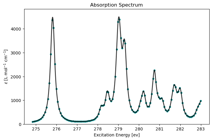
Text file
@jobs
task: response
@end

@method settings
xcfun: cam-b3lyp
basis: def2-svp
@end

@response
property: absorption (cpp)
# frequency region (and resolution)
frequencies: 10.1-10.4 (0.0025)
@end

@molecule
charge: 0
multiplicity: 1
xyz:
...
@end
Please refer to the keyword list for a complete set of CPP options.
RIXS
RIXS is a photon-in−photon-out technique which transfers the element- and site-selectivity of XAS to the valence-excited state manifold. The double differential scattering cross-section corresponding to the electronic inelastic process is described within the Kramers-Heisenberg-Dirac (KHD) formulation:
Here, ℏω and ℏω′ are the incoming, respectively outgoing photon energies, ∣0⟩ is the electronic ground state, ∣f⟩ is a final valence-excited state, ∣n⟩ is an intermediate core-excited state and ℏω0, ℏωf, and ℏωn are their respective energies. The constants re and me are the classical electron radius, respectively the electron mass, while ε and ε′ are, respectively, the incoming and outgoing polarization vectors. Γn is the full-width-at-half-maximum lifetime broadening of the core-excited intermediate state ∣n⟩.
Although computing RIXS scattering cross-sections formally requires quadratic response for the core-to-valence transition dipole moments, these second-order matrix elements may be approximated at first-order similarly as, e.g., for excited-state absorption. In this approach, the scattering cross-sections can be determined from two TDDFT calculations, one to obtain the valence-excited states and the other to obtain the core-excited states. The state-to-state transition density matrices are then computed using the linear-response (LR) eigenvectors. A detailed discussion of the theory, as well as a benchmark of the VeloxChem LR-TDDFT implementaion can be found in Vitols et al. (2025).
RIXS calculations can be performed using the RixsDriver, as shown below.
Python script
import veloxchem as vlx

molecule = vlx.Molecule.read_xyz_string("""13
ESCA b3lyp/def2-svp optimized geometry
C              1.326024532622         0.471089167011        -1.154937296389
C              0.484399509715         0.908494386259         0.037569541020
C              0.270494167717        -0.188493907246         1.053914467110
O              0.701245126416        -1.308212251798         0.971080711541
C             -0.582260522270         0.210893702941         2.291730106998
F             -0.731967860619        -0.799813015071         3.135965340271
F             -1.800383044157         0.625073687043         1.897202571864
F              0.003899498844         1.231896946553         2.943599980006
H              1.453639490166         1.302028888463        -1.864264306255
H              0.853135331881        -0.368249103011        -1.686230702784
H              2.322713498820         0.134038471332        -0.833394707486
H              0.936346512410         1.764030447212         0.571699332428
H             -0.514670521097         1.267150587304        -0.270103071648""")

basis = vlx.MolecularBasis.read(molecule, "def2-svp")

xcfun = "cam-b3lyp"

scf_drv = vlx.ScfRestrictedDriver()
scf_drv.xcfun = xcfun
scf_results = scf_drv.compute(molecule, basis)

rixs_drv = vlx.RixsDriver()
rixs_drv.nstates = 20   # number of final valence-excited states
rixs_drv.num_core_orbitals = 8   # number of core orbitals
rixs_drv.num_core_states = 10  # number of intermediate core-excited states

rixs_drv.photon_energy = 276 / vlx.hartree_in_ev()  # value of the incoming photon energy in a.u.

rixs_results = rixs_drv.compute(molecule, basis, scf_results)
Self Consistent Field Driver Setup
====================================
Wave Function Model : Spin-Restricted Kohn-Sham
Initial Guess Model : Superposition of Atomic Densities
Convergence Accelerator : Two Level Direct Inversion of Iterative Subspace
Max. Number of Iterations : 50
Max. Number of Error Vectors : 10
Convergence Threshold : 1.0e-06
ERI Screening Threshold : 1.0e-12
Linear Dependence Threshold : 1.0e-06
Exchange-Correlation Functional : CAM-B3LYP
Molecular Grid Level : 4
* Info * Using the CAM-B3LYP functional.
T. Yanai, D. P. Tew, and N. C. Handy., Chem. Phys. Lett. 393, 51 (2004)
* Info * Using the Libxc library (v7.0.0).
S. Lehtola, C. Steigemann, M. J.T. Oliveira, and M. A.L. Marques., SoftwareX 7, 1–5 (2018)
* Info * Using the following algorithm for XC numerical integration.
J. Kussmann, H. Laqua and C. Ochsenfeld, J. Chem. Theory Comput. 2021, 17, 1512-1521
* Info * Starting Reduced Basis SCF calculation...
* Info * ...done. SCF energy in reduced basis set: -526.938455740283 a.u. Time: 0.73 sec.
Iter. | Kohn-Sham Energy | Energy Change | Gradient Norm | Max. Gradient | Density Change
--------------------------------------------------------------------------------------------
1 -529.586728466450 0.0000000000 0.53374620 0.03593589 0.00000000
2 -529.603124499109 -0.0163960327 0.34722120 0.01846824 0.24699450
3 -529.612890240900 -0.0097657418 0.11504978 0.00660439 0.11657923
4 -529.613961545143 -0.0010713042 0.02982386 0.00173799 0.03726681
5 -529.614036248886 -0.0000747037 0.00809739 0.00064678 0.01189255
6 -529.614042270130 -0.0000060212 0.00116613 0.00004845 0.00281801
7 -529.614042478615 -0.0000002085 0.00038410 0.00002043 0.00090265
8 -529.614042496457 -0.0000000178 0.00012919 0.00000627 0.00018292
9 -529.614042498602 -0.0000000021 0.00004534 0.00000240 0.00009678
10 -529.614042498793 -0.0000000002 0.00001186 0.00000045 0.00002019
11 -529.614042498810 -0.0000000000 0.00000290 0.00000015 0.00000634
12 -529.614042498811 -0.0000000000 0.00000064 0.00000003 0.00000258
*** SCF converged in 12 iterations. Time: 18.85 sec.
Spin-Restricted Kohn-Sham:
--------------------------
Total Energy : -529.6140424988 a.u.
Electronic Energy : -939.5241314647 a.u.
Nuclear Repulsion Energy : 409.9100889659 a.u.
------------------------------------
Gradient Norm : 0.0000006381 a.u.
Ground State Information
------------------------
Charge of Molecule : 0.0
Multiplicity (2S+1) : 1
Magnetic Quantum Number (M_S) : 0.0
Linear Response EigenSolver Setup
===================================
Number of States : 20
Max. Number of Iterations : 150
Convergence Threshold : 2.0e-05
ERI Screening Threshold : 1.0e-12
Exchange-Correlation Functional : CAM-B3LYP
Molecular Grid Level : 4
* Info * Using the CAM-B3LYP functional.
T. Yanai, D. P. Tew, and N. C. Handy., Chem. Phys. Lett. 393, 51 (2004)
* Info * Using the Libxc library (v7.0.0).
S. Lehtola, C. Steigemann, M. J.T. Oliveira, and M. A.L. Marques., SoftwareX 7, 1–5 (2018)
* Info * Using the following algorithm for XC numerical integration.
J. Kussmann, H. Laqua and C. Ochsenfeld, J. Chem. Theory Comput. 2021, 17, 1512-1521
* Info * 40 gerade trial vectors in reduced space
* Info * 40 ungerade trial vectors in reduced space
*** Iteration: 1 * Residuals (Max,Min): 2.88e-01 and 7.21e-02
* Info * 60 gerade trial vectors in reduced space
* Info * 60 ungerade trial vectors in reduced space
*** Iteration: 2 * Residuals (Max,Min): 8.75e-02 and 2.09e-02
* Info * 80 gerade trial vectors in reduced space
* Info * 80 ungerade trial vectors in reduced space
*** Iteration: 3 * Residuals (Max,Min): 2.22e-02 and 3.39e-03
* Info * 100 gerade trial vectors in reduced space
* Info * 100 ungerade trial vectors in reduced space
*** Iteration: 4 * Residuals (Max,Min): 6.82e-03 and 5.15e-04
* Info * 120 gerade trial vectors in reduced space
* Info * 120 ungerade trial vectors in reduced space
*** Iteration: 5 * Residuals (Max,Min): 2.17e-03 and 6.72e-05
* Info * 140 gerade trial vectors in reduced space
* Info * 140 ungerade trial vectors in reduced space
*** Iteration: 6 * Residuals (Max,Min): 5.02e-04 and 6.54e-06
* Info * 158 gerade trial vectors in reduced space
* Info * 158 ungerade trial vectors in reduced space
*** Iteration: 7 * Residuals (Max,Min): 1.17e-04 and 2.63e-06
* Info * 167 gerade trial vectors in reduced space
* Info * 167 ungerade trial vectors in reduced space
*** Iteration: 8 * Residuals (Max,Min): 2.89e-05 and 1.63e-06
* Info * 171 gerade trial vectors in reduced space
* Info * 171 ungerade trial vectors in reduced space
*** Iteration: 9 * Residuals (Max,Min): 1.37e-05 and 1.62e-06
*** Linear response converged in 9 iterations. Time: 246.63 sec
Electric Transition Dipole Moments (dipole length, a.u.)
--------------------------------------------------------
X Y Z
Excited State S1: 0.018446 0.006267 0.010778
Excited State S2: -0.085492 -0.038045 -0.046010
Excited State S3: 0.034113 -0.531657 0.258415
Excited State S4: -0.005242 -0.001612 -0.002974
Excited State S5: -0.046150 -0.078380 0.126414
Excited State S6: 0.036536 0.012459 0.021264
Excited State S7: -0.243176 0.579583 0.078125
Excited State S8: 0.017227 -0.086354 0.021169
Excited State S9: -0.179256 -0.067619 -0.105898
Excited State S10: 0.017939 0.006500 0.008935
Excited State S11: -0.109979 0.321329 -0.007699
Excited State S12: -0.089866 -0.042783 0.180982
Excited State S13: -0.061714 -0.020744 -0.035561
Excited State S14: 0.070634 0.024172 0.040876
Excited State S15: -0.151311 -0.184857 0.369554
Excited State S16: -0.052542 -0.314143 0.275480
Excited State S17: -0.020923 0.145099 -0.048154
Excited State S18: -0.236647 -0.163741 0.507178
Excited State S19: -0.011252 -0.007526 0.012794
Excited State S20: 0.092274 0.031561 0.051482
Electric Transition Dipole Moments (dipole velocity, a.u.)
----------------------------------------------------------
X Y Z
Excited State S1: 0.016581 0.005693 0.009844
Excited State S2: -0.078216 -0.034580 -0.042532
Excited State S3: 0.039198 -0.471831 0.214046
Excited State S4: -0.014660 -0.004756 -0.008407
Excited State S5: -0.045550 -0.090405 0.132483
Excited State S6: 0.080024 0.027256 0.046557
Excited State S7: -0.215787 0.524136 0.063552
Excited State S8: 0.009760 -0.107420 0.046595
Excited State S9: -0.189426 -0.071328 -0.111395
Excited State S10: 0.020434 0.007222 0.010383
Excited State S11: -0.103031 0.342917 -0.032802
Excited State S12: -0.079571 -0.064671 0.175487
Excited State S13: -0.061366 -0.020740 -0.035332
Excited State S14: 0.089791 0.030859 0.051918
Excited State S15: -0.137188 -0.152486 0.326206
Excited State S16: -0.051026 -0.347882 0.292795
Excited State S17: -0.001722 0.127944 -0.071546
Excited State S18: -0.237877 -0.235439 0.553631
Excited State S19: -0.043020 -0.020352 -0.004438
Excited State S20: 0.090841 0.031823 0.050463
Magnetic Transition Dipole Moments (a.u.)
-----------------------------------------
X Y Z
Excited State S1: -0.219522 0.493806 0.087617
Excited State S2: -0.124457 -0.139753 0.303834
Excited State S3: 0.218406 0.025904 0.009103
Excited State S4: 0.135677 0.045780 -0.261353
Excited State S5: -0.087753 -0.063533 -0.073842
Excited State S6: -0.231461 -0.010574 0.405449
Excited State S7: -0.215919 -0.091186 0.019678
Excited State S8: 0.026895 -0.003575 -0.014087
Excited State S9: 0.020088 -0.034859 -0.007472
Excited State S10: -0.067597 0.054340 0.084759
Excited State S11: -0.189081 -0.055971 -0.008516
Excited State S12: -0.033828 -0.063305 -0.037749
Excited State S13: 0.094974 -0.308603 0.018703
Excited State S14: -0.142735 -0.345290 0.451049
Excited State S15: 0.319200 0.009361 0.137680
Excited State S16: -0.383654 -0.224028 -0.332844
Excited State S17: -0.180579 -0.038827 -0.064015
Excited State S18: -0.188723 -0.243365 -0.190568
Excited State S19: -0.066721 -0.049324 0.124769
Excited State S20: -0.102159 0.049993 0.152313
One-Photon Absorption
---------------------
Excited State S1: 0.16001143 a.u. 4.35413 eV Osc.Str. 0.0001
Excited State S2: 0.30585617 a.u. 8.32277 eV Osc.Str. 0.0022
Excited State S3: 0.30639564 a.u. 8.33745 eV Osc.Str. 0.0716
Excited State S4: 0.31620144 a.u. 8.60428 eV Osc.Str. 0.0000
Excited State S5: 0.32961040 a.u. 8.96916 eV Osc.Str. 0.0053
Excited State S6: 0.34837638 a.u. 9.47980 eV Osc.Str. 0.0005
Excited State S7: 0.35673130 a.u. 9.70715 eV Osc.Str. 0.0954
Excited State S8: 0.36197627 a.u. 9.84988 eV Osc.Str. 0.0020
Excited State S9: 0.37976961 a.u. 10.33406 eV Osc.Str. 0.0121
Excited State S10: 0.38051727 a.u. 10.35440 eV Osc.Str. 0.0001
Excited State S11: 0.38124094 a.u. 10.37409 eV Osc.Str. 0.0293
Excited State S12: 0.38276874 a.u. 10.41567 eV Osc.Str. 0.0109
Excited State S13: 0.38783382 a.u. 10.55350 eV Osc.Str. 0.0014
Excited State S14: 0.38856884 a.u. 10.57350 eV Osc.Str. 0.0019
Excited State S15: 0.39831855 a.u. 10.83880 eV Osc.Str. 0.0514
Excited State S16: 0.41066241 a.u. 11.17469 eV Osc.Str. 0.0486
Excited State S17: 0.41332900 a.u. 11.24726 eV Osc.Str. 0.0066
Excited State S18: 0.42078449 a.u. 11.45013 eV Osc.Str. 0.0954
Excited State S19: 0.42135857 a.u. 11.46575 eV Osc.Str. 0.0001
Excited State S20: 0.42260587 a.u. 11.49969 eV Osc.Str. 0.0034
Electronic Circular Dichroism
-----------------------------
Excited State S1: Rot.Str. 0.000034 a.u. 0.0160 [10**(-40) cgs]
Excited State S2: Rot.Str. 0.001644 a.u. 0.7752 [10**(-40) cgs]
Excited State S3: Rot.Str. -0.001713 a.u. -0.8075 [10**(-40) cgs]
Excited State S4: Rot.Str. -0.000010 a.u. -0.0046 [10**(-40) cgs]
Excited State S5: Rot.Str. -0.000042 a.u. -0.0197 [10**(-40) cgs]
Excited State S6: Rot.Str. 0.000066 a.u. 0.0310 [10**(-40) cgs]
Excited State S7: Rot.Str. 0.000049 a.u. 0.0232 [10**(-40) cgs]
Excited State S8: Rot.Str. -0.000010 a.u. -0.0046 [10**(-40) cgs]
Excited State S9: Rot.Str. -0.000486 a.u. -0.2293 [10**(-40) cgs]
Excited State S10: Rot.Str. -0.000109 a.u. -0.0513 [10**(-40) cgs]
Excited State S11: Rot.Str. 0.000567 a.u. 0.2673 [10**(-40) cgs]
Excited State S12: Rot.Str. 0.000161 a.u. 0.0761 [10**(-40) cgs]
Excited State S13: Rot.Str. -0.000089 a.u. -0.0417 [10**(-40) cgs]
Excited State S14: Rot.Str. -0.000054 a.u. -0.0255 [10**(-40) cgs]
Excited State S15: Rot.Str. -0.000306 a.u. -0.1442 [10**(-40) cgs]
Excited State S16: Rot.Str. 0.000057 a.u. 0.0269 [10**(-40) cgs]
Excited State S17: Rot.Str. -0.000077 a.u. -0.0362 [10**(-40) cgs]
Excited State S18: Rot.Str. -0.003314 a.u. -1.5624 [10**(-40) cgs]
Excited State S19: Rot.Str. 0.003320 a.u. 1.5654 [10**(-40) cgs]
Excited State S20: Rot.Str. -0.000003 a.u. -0.0015 [10**(-40) cgs]
Character of excitations:
Excited state 1
---------------
HOMO -> LUMO 0.9901
Excited state 2
---------------
HOMO-3 -> LUMO 0.6873
HOMO-2 -> LUMO 0.6412
HOMO-6 -> LUMO 0.2832
Excited state 3
---------------
HOMO-1 -> LUMO 0.9830
Excited state 4
---------------
HOMO-3 -> LUMO 0.6500
HOMO-2 -> LUMO -0.6452
HOMO-9 -> LUMO -0.3226
Excited state 5
---------------
HOMO -> LUMO+1 -0.9581
Excited state 6
---------------
HOMO-6 -> LUMO 0.8682
HOMO-2 -> LUMO -0.3190
HOMO-9 -> LUMO 0.2695
Excited state 7
---------------
HOMO-4 -> LUMO 0.9336
HOMO -> LUMO+6 -0.2456
Excited state 8
---------------
HOMO-5 -> LUMO 0.9928
Excited state 9
---------------
HOMO -> LUMO+3 -0.9799
Excited state 10
----------------
HOMO-8 -> LUMO -0.9548
Excited state 11
----------------
HOMO -> LUMO+2 -0.9136
HOMO -> LUMO+6 0.3202
Excited state 12
----------------
HOMO-7 -> LUMO 0.9799
Excited state 13
----------------
HOMO-1 -> LUMO+1 -0.6413
HOMO-9 -> LUMO -0.6271
HOMO-6 -> LUMO 0.2457
Excited state 14
----------------
HOMO-1 -> LUMO+1 -0.7493
HOMO-9 -> LUMO 0.5406
HOMO-6 -> LUMO -0.2154
Excited state 15
----------------
HOMO -> LUMO+6 -0.7143
HOMO -> LUMO+4 -0.5241
HOMO -> LUMO+2 -0.3242
Excited state 16
----------------
HOMO-2 -> LUMO+1 0.9462
HOMO -> LUMO+4 -0.2480
Excited state 17
----------------
HOMO-10 -> LUMO 0.8815
HOMO -> LUMO+4 0.3760
Excited state 18
----------------
HOMO -> LUMO+4 -0.5607
HOMO-3 -> LUMO+1 -0.4873
HOMO -> LUMO+6 0.3759
HOMO-10 -> LUMO 0.3750
HOMO-12 -> LUMO -0.2116
Excited state 19
----------------
HOMO -> LUMO+5 0.9491
HOMO-11 -> LUMO 0.2011
Excited state 20
----------------
HOMO-11 -> LUMO 0.9194
HOMO-9 -> LUMO -0.2982
Linear Response EigenSolver Setup
===================================
Number of States : 10
Max. Number of Iterations : 150
Convergence Threshold : 2.0e-05
ERI Screening Threshold : 1.0e-12
Exchange-Correlation Functional : CAM-B3LYP
Molecular Grid Level : 4
* Info * Using the CAM-B3LYP functional.
T. Yanai, D. P. Tew, and N. C. Handy., Chem. Phys. Lett. 393, 51 (2004)
* Info * Using the Libxc library (v7.0.0).
S. Lehtola, C. Steigemann, M. J.T. Oliveira, and M. A.L. Marques., SoftwareX 7, 1–5 (2018)
* Info * Using the following algorithm for XC numerical integration.
J. Kussmann, H. Laqua and C. Ochsenfeld, J. Chem. Theory Comput. 2021, 17, 1512-1521
* Info * 30 gerade trial vectors in reduced space
* Info * 30 ungerade trial vectors in reduced space
*** Iteration: 1 * Residuals (Max,Min): 1.13e-01 and 2.87e-02
* Info * 40 gerade trial vectors in reduced space
* Info * 40 ungerade trial vectors in reduced space
*** Iteration: 2 * Residuals (Max,Min): 2.76e-02 and 2.56e-03
* Info * 50 gerade trial vectors in reduced space
* Info * 50 ungerade trial vectors in reduced space
*** Iteration: 3 * Residuals (Max,Min): 9.12e-03 and 3.50e-04
* Info * 60 gerade trial vectors in reduced space
* Info * 60 ungerade trial vectors in reduced space
*** Iteration: 4 * Residuals (Max,Min): 1.36e-03 and 2.85e-05
* Info * 69 gerade trial vectors in reduced space
* Info * 70 ungerade trial vectors in reduced space
*** Iteration: 5 * Residuals (Max,Min): 2.67e-04 and 4.12e-06
* Info * 75 gerade trial vectors in reduced space
* Info * 76 ungerade trial vectors in reduced space
*** Iteration: 6 * Residuals (Max,Min): 3.03e-05 and 1.09e-06
* Info * 77 gerade trial vectors in reduced space
* Info * 77 ungerade trial vectors in reduced space
*** Iteration: 7 * Residuals (Max,Min): 1.83e-05 and 5.22e-07
*** Linear response converged in 7 iterations. Time: 109.37 sec
Electric Transition Dipole Moments (dipole length, a.u.)
--------------------------------------------------------
X Y Z
Excited State S1: 0.003397 0.001165 0.001963
Excited State S2: 0.076544 0.026165 0.044342
Excited State S3: -0.000613 -0.000217 -0.000382
Excited State S4: -0.012904 -0.002821 0.023932
Excited State S5: -0.017983 0.037065 0.009101
Excited State S6: -0.007424 0.059446 -0.021063
Excited State S7: 0.050243 0.016571 0.029284
Excited State S8: -0.058341 -0.020055 -0.033793
Excited State S9: 0.005412 -0.018110 0.001368
Excited State S10: -0.005673 -0.025207 0.024887
Electric Transition Dipole Moments (dipole velocity, a.u.)
----------------------------------------------------------
X Y Z
Excited State S1: 0.002559 0.000877 0.001477
Excited State S2: 0.075486 0.025801 0.043728
Excited State S3: -0.000701 -0.000246 -0.000432
Excited State S4: -0.013032 -0.002560 0.024002
Excited State S5: -0.018241 0.038054 0.008960
Excited State S6: -0.008128 0.060877 -0.020667
Excited State S7: 0.051349 0.016933 0.029918
Excited State S8: -0.059357 -0.020406 -0.034389
Excited State S9: 0.003568 -0.017000 0.003890
Excited State S10: -0.003800 -0.026934 0.022683
Magnetic Transition Dipole Moments (a.u.)
-----------------------------------------
X Y Z
Excited State S1: 0.010933 -0.003756 -0.016712
Excited State S2: -0.342094 0.650371 0.206796
Excited State S3: -0.005214 0.014144 0.000435
Excited State S4: 0.077461 -0.162992 0.024670
Excited State S5: 0.063606 -0.048989 0.337563
Excited State S6: 0.589396 0.357009 0.820557
Excited State S7: 0.328342 -0.985564 -0.005099
Excited State S8: -0.296746 0.161370 0.416526
Excited State S9: -0.174220 -0.090582 -0.236020
Excited State S10: 0.207536 -0.109095 -0.094768
One-Photon Absorption
---------------------
Excited State S1: 10.12438061 a.u. 275.49843 eV Osc.Str. 0.0001
Excited State S2: 10.14146367 a.u. 275.96328 eV Osc.Str. 0.0575
Excited State S3: 10.14639446 a.u. 276.09746 eV Osc.Str. 0.0000
Excited State S4: 10.21531301 a.u. 277.97283 eV Osc.Str. 0.0051
Excited State S5: 10.22775121 a.u. 278.31129 eV Osc.Str. 0.0121
Excited State S6: 10.24946857 a.u. 278.90225 eV Osc.Str. 0.0276
Excited State S7: 10.25098734 a.u. 278.94358 eV Osc.Str. 0.0250
Excited State S8: 10.25942128 a.u. 279.17308 eV Osc.Str. 0.0338
Excited State S9: 10.27791314 a.u. 279.67626 eV Osc.Str. 0.0025
Excited State S10: 10.28757003 a.u. 279.93904 eV Osc.Str. 0.0088
Electronic Circular Dichroism
-----------------------------
Excited State S1: Rot.Str. -0.000000 a.u. -0.0000 [10**(-40) cgs]
Excited State S2: Rot.Str. -0.000000 a.u. -0.0000 [10**(-40) cgs]
Excited State S3: Rot.Str. -0.000000 a.u. -0.0000 [10**(-40) cgs]
Excited State S4: Rot.Str. -0.000000 a.u. -0.0000 [10**(-40) cgs]
Excited State S5: Rot.Str. 0.000000 a.u. 0.0000 [10**(-40) cgs]
Excited State S6: Rot.Str. -0.000016 a.u. -0.0074 [10**(-40) cgs]
Excited State S7: Rot.Str. 0.000019 a.u. 0.0088 [10**(-40) cgs]
Excited State S8: Rot.Str. -0.000003 a.u. -0.0013 [10**(-40) cgs]
Excited State S9: Rot.Str. 0.000000 a.u. 0.0000 [10**(-40) cgs]
Excited State S10: Rot.Str. 0.000000 a.u. 0.0000 [10**(-40) cgs]
Character of excitations:
Excited state 1
---------------
core_7 -> LUMO -0.9971
Excited state 2
---------------
core_6 -> LUMO 0.9939
Excited state 3
---------------
core_8 -> LUMO 0.9983
Excited state 4
---------------
core_8 -> LUMO+1 0.9636
Excited state 5
---------------
core_7 -> LUMO+1 -0.9526
core_7 -> LUMO+2 0.2392
Excited state 6
---------------
core_8 -> LUMO+4 0.8748
core_8 -> LUMO+2 0.4631
Excited state 7
---------------
core_8 -> LUMO+3 -0.8061
core_8 -> LUMO+5 -0.5788
Excited state 8
---------------
core_7 -> LUMO+3 0.9602
core_7 -> LUMO+5 -0.2267
Excited state 9
---------------
core_8 -> LUMO+2 0.8548
core_8 -> LUMO+4 -0.4474
Excited state 10
----------------
core_7 -> LUMO+2 -0.9095
core_7 -> LUMO+8 0.2090
core_7 -> LUMO+1 -0.2063
Resonant Inelastic X-ray Scattering (RIXS) Setup
================================================
Scattering angle (theta) [rad] : 0.00
Lifetime broadening (gamma) [eV] : 0.12
Incoming photon energies [a.u.] : 10.1428
Incoming photon energies [eV] : 276.00
Number of intermediate states : 10
Number of final states : 20
State index sets
Intermediate/core states : [0 ... 9]
Final/valence states : [0 ... 19]
Orbital sets
Core orbitals : [Core1 ... Core8]
Valence orbitals : [HOMO-23 ... HOMO]
Virtual orbitals : [LUMO ... LUMO+104]
* Info * Running RIXS calculation in the two-shot approach
J. Phys. Chem. A, 2025, 129, 8783-8797, DOI: 10.1021/acs.jpca.5c04528
* Info * Computed RIXS cross-sections for 20 final states at photon energy: 276.00 eV.
RIXS cross-sections at incident X-ray energy 276.00 eV, energy-loss mode
------------------------------------------------------------------------
Ground State S0: 0.00000000 a.u. 0.00000 eV Cross-section 2.04e-05
Excited State S1: 0.16001143 a.u. 4.35413 eV Cross-section 1.25e-06
Excited State S2: 0.30585617 a.u. 8.32277 eV Cross-section 4.91e-06
Excited State S3: 0.30639564 a.u. 8.33745 eV Cross-section 5.41e-08
Excited State S4: 0.31620144 a.u. 8.60428 eV Cross-section 7.66e-06
Excited State S5: 0.32961040 a.u. 8.96916 eV Cross-section 4.18e-08
Excited State S6: 0.34837638 a.u. 9.47980 eV Cross-section 5.63e-06
Excited State S7: 0.35673130 a.u. 9.70715 eV Cross-section 2.56e-06
Excited State S8: 0.36197627 a.u. 9.84988 eV Cross-section 6.23e-10
Excited State S9: 0.37976961 a.u. 10.33406 eV Cross-section 8.83e-09
Excited State S10: 0.38051727 a.u. 10.35440 eV Cross-section 3.79e-07
Excited State S11: 0.38124094 a.u. 10.37409 eV Cross-section 2.50e-08
Excited State S12: 0.38276874 a.u. 10.41567 eV Cross-section 2.24e-08
Excited State S13: 0.38783382 a.u. 10.55350 eV Cross-section 1.14e-06
Excited State S14: 0.38856884 a.u. 10.57350 eV Cross-section 8.85e-07
Excited State S15: 0.39831855 a.u. 10.83880 eV Cross-section 1.53e-08
Excited State S16: 0.41066241 a.u. 11.17469 eV Cross-section 5.40e-09
Excited State S17: 0.41332900 a.u. 11.24726 eV Cross-section 4.05e-07
Excited State S18: 0.42078449 a.u. 11.45013 eV Cross-section 2.88e-08
Excited State S19: 0.42135857 a.u. 11.46575 eV Cross-section 2.97e-08
Excited State S20: 0.42260587 a.u. 11.49969 eV Cross-section 8.55e-09
rixs_drv.plot(rixs_results)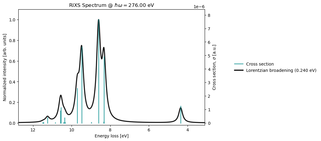
Text file
@jobs
task: response
@end

@method settings
xcfun: cam-b3lyp
basis: def2-svp
@end

@response
property: rixs
photon_energy: 10.106 - 10.290 (0.004)
nstates: 20
num_core_orbitals: 8
num_core_states: 10
@end

@molecule
charge: 0
multiplicity: 1
xyz:
...
@end
The results obtained using the input file above can be plotted in a Jupyter notebook, by reading the output from the corresponding HDF5 checkpoint file. If multiple, equally-spaced, incoming photon energies have been included, as in the example above, the results can be plotted as a 2D RIXS map. RixsDriver.plot can then be used to display cuts through the 2D map at specific photon energies.
molecule, basis = vlx.read_molecule_and_basis("../output_files/esca-rixs.h5")
rixs_results = vlx.read_results("../output_files/esca-rixs.h5", "rsp")
rixs_drv.plot_map(rixs_results)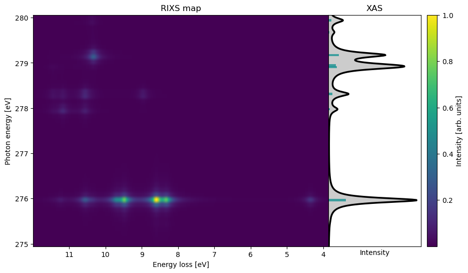
rixs_drv.plot(rixs_results, photon_energy_ev=278.5)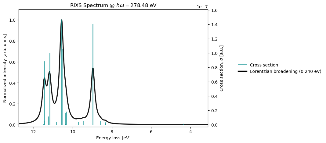
- Norman, P., & Dreuw, A. (2018). Simulating X-ray Spectroscopies and Calculating Core-Excited States of Molecules. Chem. Rev., 118(15), 7208–7248. 10.1021/acs.chemrev.8b00156
- Brumboiu, I. E., & Fransson, T. (2022). Core–hole delocalization for modeling x-ray spectroscopies: A cautionary tale. J. Chem. Phys., 156(21). 10.1063/5.0088195
- Ekström, U., & Norman, P. (2006). X-ray absorption spectra from the resonant-convergent first-order polarization propagator approach. Phys. Rev. A, 74(4), 042722. 10.1103/PhysRevA.74.042722
- Fransson, T., Brumboiu, I. E., Vidal, M. L., Norman, P., Coriani, S., & Dreuw, A. (2021). XABOOM: An X-ray Absorption Benchmark of Organic Molecules Based on Carbon, Nitrogen, and Oxygen 1s → π* Transitions. J. Chem. Theory Comput., 17(3), 1618–1637. 10.1021/acs.jctc.0c01082
- Vitols, E., Vaz da Cruz, V., Fransson, T., & Brumboiu, I. E. (2025). Resonant Inelastic X-ray Scattering: How Well Does LR-TDDFT Perform? J. Phys. Chem. A, 129(38), 8783–8797. 10.1021/acs.jpca.5c04528