Multi-photon interactions describe the nonlinear responses of a molecular system to the simultaneous absorption or emission of two or more photons. These processes arise from higher‑order terms in the light–matter interaction and are governed by electronic transition pathways that do not appear in linear spectroscopy. Within the Born–Oppenheimer and electric‑dipole approximations, multi-photon effects are characterized by frequency‑dependent response functions—such as second‑ and third‑order polarizabilities—that encode resonant enhancements and selection rules beyond those of one‑photon transitions.
VeloxChem provides efficient tools for computing these nonlinear response properties at the levels of time‑dependent density functional theory (TDDFT) and the complex polarization propagator (CPP) aproach. By solving perturbation‑dependent response equations for multiple field frequencies, the program enables the evaluation of two‑photon absorption amplitudes, hyperpolarizabilities, and other nonlinear optical indicators relevant to multi-photon spectroscopies.
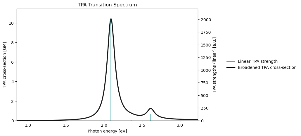
In the quadratic response theory framework, two‑photon absorption (TPA) spectra are determined from residues of the second‑order response function at half the excitation energy. TPA strengths factorize into products of transition moments, which quantify the effective coupling of the ground state to an excited state via the simultaneous interaction with two photons. The two-photon transition moment is given by the sum-over-states expression
where ℏωn0 is the excitation energy for state ∣n⟩, μ^α is the electric dipole moment operator along the Cartesian axis α , and the summation includes the ground state, ∣n⟩=∣0⟩.
For an isotropic sample, the experimentally relevant TPA strengths are obtained from the orientational average of the squared magnitudes of the Cartesian transition moments. This averaging yields a scalar measure that captures the laser field polarization, and it provides the quantity directly comparable to measured TPA cross sections, see Norman et al. (2018) for further details.
where α is the fine structure constant, a0 is the Bohr radius, c is the speed of light, and g is a line broadening function with unit area centered at half the transition angular frequency ωf0/2 and dependent on the dampening parameter γ. Specific for the Lorentzian broadening function, its value at a TP resonance frequency (2ω=ωf0) is equal to
The unit of the cross section will be GM (after Maria Göppert-Mayer) given that atomic units is used for ω, δfTPA, and g and SI units is used for the rest, and that a multiplication by a factor of 1058 is made to account for the fact that 1 GM corresponds to 10-50 cm4s photon−1.
TPA simulations are sensitive toward the choice of basis set and exchange-correlation functional. The inclusion of diffuse functions in the basis set is typically required, and in regard with functionals, it has been demonstrated that the range-separated hybrid CAM-B3LYP and the hybrid meta-GGA MN15 functionals are good choices, see Ahmadzadeh et al. (2024).
                                            Self Consistent Field Driver Setup
                                           ====================================

                   Wave Function Model             : Spin-Restricted Kohn-Sham
                   Initial Guess Model             : Superposition of Atomic Densities
                   Convergence Accelerator         : Two Level Direct Inversion of Iterative Subspace
                   Max. Number of Iterations       : 50
                   Max. Number of Error Vectors    : 10
                   Convergence Threshold           : 1.0e-06
                   ERI Screening Threshold         : 1.0e-12
                   Linear Dependence Threshold     : 1.0e-06
                   Exchange-Correlation Functional : CAM-B3LYP
                   Molecular Grid Level            : 4

* Info * Using the CAM-B3LYP functional.

         T. Yanai, D. P. Tew, and N. C. Handy.,  Chem. Phys. Lett. 393, 51 (2004)

* Info * Using the Libxc library (v7.0.0).

         S. Lehtola, C. Steigemann, M. J.T. Oliveira, and M. A.L. Marques.,  SoftwareX 7, 1–5 (2018)

* Info * Using the following algorithm for XC numerical integration.

         J. Kussmann, H. Laqua and C. Ochsenfeld, J. Chem. Theory Comput. 2021, 17, 1512-1521

* Info * Starting Reduced Basis SCF calculation...
* Info * ...done. SCF energy in reduced basis set: -488.569243820879 a.u. Time: 0.47 sec.


               Iter. |    Kohn-Sham Energy | Energy Change | Gradient Norm | Max. Gradient | Density Change
               --------------------------------------------------------------------------------------------
                  1      -491.466830345380    0.0000000000      0.44818638      0.03253433      0.00000000
                  2      -491.467030233471   -0.0001998881      0.47878777      0.02894784      0.28466471
                  3      -491.488003622382   -0.0209733889      0.12797776      0.00869974      0.14515176
                  4      -491.489393491948   -0.0013898696      0.04064637      0.00378322      0.04532806
                  5      -491.489526770776   -0.0001332788      0.02412501      0.00165159      0.01672683
                  6      -491.489587625425   -0.0000608546      0.00462731      0.00021875      0.00786242
                  7      -491.489591357225   -0.0000037318      0.00300436      0.00019584      0.00317189
                  8      -491.489592606845   -0.0000012496      0.00086635      0.00003620      0.00138467
                  9      -491.489592730362   -0.0000001235      0.00032582      0.00001823      0.00062889
                 10      -491.489592744126   -0.0000000138      0.00008203      0.00000336      0.00014903
                 11      -491.489592745223   -0.0000000011      0.00003539      0.00000199      0.00006470
                 12      -491.489592745380   -0.0000000002      0.00000767      0.00000043      0.00001630
                 13      -491.489592745390   -0.0000000000      0.00000372      0.00000016      0.00000575
                 14      -491.489592745392   -0.0000000000      0.00000123      0.00000007      0.00000256
                 15      -491.489592745391    0.0000000000      0.00000040      0.00000003      0.00000074

               *** SCF converged in 15 iterations. Time: 11.56 sec.

               Spin-Restricted Kohn-Sham:
               --------------------------
               Total Energy                       :     -491.4895927454 a.u.
               Electronic Energy                  :     -977.4903807130 a.u.
               Nuclear Repulsion Energy           :      486.0007879676 a.u.
               ------------------------------------
               Gradient Norm                      :        0.0000004024 a.u.


               Ground State Information
               ------------------------
               Charge of Molecule            :  0.0
               Multiplicity (2S+1)           :  1
               Magnetic Quantum Number (M_S) :  0.0


                                             Quadratic Response Driver Setup
                                            =================================

                                    ERI Screening Threshold         : 1.0e-12
                                    Convergance Threshold           : 1.0e-04
                                    Max. Number of Iterations       : 150
                                    Max. Number of Iterations       : 150


                                            Linear Response EigenSolver Setup
                                           ===================================

                               Number of States                : 5
                               Max. Number of Iterations       : 150
                               Convergence Threshold           : 1.0e-04
                               ERI Screening Threshold         : 1.0e-12
                               Exchange-Correlation Functional : CAM-B3LYP
                               Molecular Grid Level            : 4

* Info * Using the CAM-B3LYP functional.

         T. Yanai, D. P. Tew, and N. C. Handy.,  Chem. Phys. Lett. 393, 51 (2004)

* Info * Using the Libxc library (v7.0.0).

         S. Lehtola, C. Steigemann, M. J.T. Oliveira, and M. A.L. Marques.,  SoftwareX 7, 1–5 (2018)

* Info * Using the following algorithm for XC numerical integration.

         J. Kussmann, H. Laqua and C. Ochsenfeld, J. Chem. Theory Comput. 2021, 17, 1512-1521

* Info * 15 gerade trial vectors in reduced space
* Info * 15 ungerade trial vectors in reduced space

               *** Iteration:   1 * Residuals (Max,Min): 4.04e-01 and 9.04e-02

* Info * 20 gerade trial vectors in reduced space
* Info * 20 ungerade trial vectors in reduced space

               *** Iteration:   2 * Residuals (Max,Min): 8.73e-02 and 1.39e-02

* Info * 25 gerade trial vectors in reduced space
* Info * 25 ungerade trial vectors in reduced space

               *** Iteration:   3 * Residuals (Max,Min): 7.43e-02 and 3.10e-03

* Info * 30 gerade trial vectors in reduced space
* Info * 30 ungerade trial vectors in reduced space

               *** Iteration:   4 * Residuals (Max,Min): 5.00e-02 and 5.51e-04

* Info * 35 gerade trial vectors in reduced space
* Info * 35 ungerade trial vectors in reduced space

               *** Iteration:   5 * Residuals (Max,Min): 1.32e-02 and 1.31e-04

* Info * 40 gerade trial vectors in reduced space
* Info * 40 ungerade trial vectors in reduced space

               *** Iteration:   6 * Residuals (Max,Min): 4.32e-03 and 2.74e-05

* Info * 44 gerade trial vectors in reduced space
* Info * 44 ungerade trial vectors in reduced space

               *** Iteration:   7 * Residuals (Max,Min): 1.06e-03 and 2.58e-05

* Info * 46 gerade trial vectors in reduced space
* Info * 46 ungerade trial vectors in reduced space

               *** Iteration:   8 * Residuals (Max,Min): 2.16e-04 and 2.58e-05

* Info * 48 gerade trial vectors in reduced space
* Info * 48 ungerade trial vectors in reduced space

               *** Iteration:   9 * Residuals (Max,Min): 7.27e-05 and 2.58e-05

               *** Linear response converged in 9 iterations. Time: 38.57 sec


                                              Complex Response Solver Setup
                                             ===============================

                               Number of Frequencies           : 1
                               Max. Number of Iterations       : 150
                               Convergence Threshold           : 1.0e-04
                               ERI Screening Threshold         : 1.0e-12
                               Exchange-Correlation Functional : CAM-B3LYP
                               Molecular Grid Level            : 4

* Info * Using the CAM-B3LYP functional.

         T. Yanai, D. P. Tew, and N. C. Handy.,  Chem. Phys. Lett. 393, 51 (2004)

* Info * Using the Libxc library (v7.0.0).

         S. Lehtola, C. Steigemann, M. J.T. Oliveira, and M. A.L. Marques.,  SoftwareX 7, 1–5 (2018)

* Info * Using the following algorithm for XC numerical integration.

         J. Kussmann, H. Laqua and C. Ochsenfeld, J. Chem. Theory Comput. 2021, 17, 1512-1521

* Info * 8 gerade trial vectors in reduced space
* Info * 9 ungerade trial vectors in reduced space

               *** Iteration:   1 * Residuals (Max,Min): 1.01e+00 and 5.45e-01

* Info * 17 gerade trial vectors in reduced space
* Info * 20 ungerade trial vectors in reduced space

               *** Iteration:   2 * Residuals (Max,Min): 1.24e-01 and 8.99e-02

* Info * 28 gerade trial vectors in reduced space
* Info * 32 ungerade trial vectors in reduced space

               *** Iteration:   3 * Residuals (Max,Min): 3.98e-02 and 2.85e-02

* Info * 39 gerade trial vectors in reduced space
* Info * 44 ungerade trial vectors in reduced space

               *** Iteration:   4 * Residuals (Max,Min): 9.02e-03 and 5.55e-03

* Info * 49 gerade trial vectors in reduced space
* Info * 57 ungerade trial vectors in reduced space

               *** Iteration:   5 * Residuals (Max,Min): 2.06e-03 and 1.15e-03

* Info * 60 gerade trial vectors in reduced space
* Info * 70 ungerade trial vectors in reduced space

               *** Iteration:   6 * Residuals (Max,Min): 4.43e-04 and 1.80e-04

* Info * 70 gerade trial vectors in reduced space
* Info * 83 ungerade trial vectors in reduced space

               *** Iteration:   7 * Residuals (Max,Min): 7.35e-05 and 2.84e-05

               *** Complex response converged in 7 iterations. Time: 66.13 sec


                                                 Fock Matrix Computation
                                                =========================

* Info * Processing 20 Fock builds...

* Info * Time spent in Fock matrices: 16.95 sec

                             *** Time spent in quadratic response calculation: 122.05 sec ***


                                             Summary of Two-photon Absorption
                                            ==================================


                                       Components of TPA Transition Moments (a.u.)
               --------------------------------------------------------------------------------------------
                 State    Photon Energy      Sxx        Syy        Szz        Sxy        Sxz        Syz
               --------------------------------------------------------------------------------------------
                     1      1.472774 eV    -0.1083     0.1087    -0.0004    -0.0776     0.1268    -0.0651
                     2      1.923271 eV    -0.1530    -0.4620     0.6150    -0.2676     0.0478     0.0219
                     3      2.091274 eV     3.0894   -52.7182   -45.8275   -14.0081   -10.4953   -50.1528
                     4      2.355365 eV     1.3722     0.8499     2.5872     2.4595     2.6274     1.7482
                     5      2.615234 eV    -1.2403   -10.6553   -11.9631    -6.1237    -5.5846   -11.4025


                                            TPA Strength (Linear Polarization)
               --------------------------------------------------------------------------------------------
                 State    Photon Energy            TPA strength
               --------------------------------------------------------------------------------------------
                     1      1.472774 eV            0.010167 a.u.
                     2      1.923271 eV            0.101851 a.u.
                     3      2.091274 eV         2011.763815 a.u.
                     4      2.355365 eV            7.050736 a.u.
                     5      2.615234 eV          125.361018 a.u.


                                           TPA Strength (Circular Polarization)
               --------------------------------------------------------------------------------------------
                 State    Photon Energy            TPA strength
               --------------------------------------------------------------------------------------------
                     1      1.472774 eV            0.015251 a.u.
                     2      1.923271 eV            0.152777 a.u.
                     3      2.091274 eV         1498.996500 a.u.
                     4      2.355365 eV            6.721244 a.u.
                     5      2.615234 eV           93.169726 a.u.
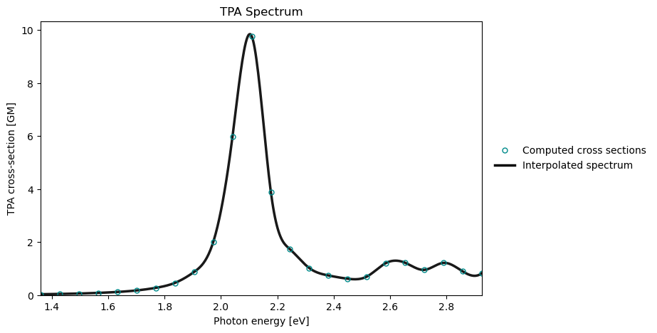
An alternative route to two-photon absorption spectra is provided by complex cubic response theoryFahleson & Norman (2017), in which the response equations are solved in the presence of a phenomenological damping parameter. Rather than evaluating individual two-photon transition moments and constructing the spectrum from discrete transitions, the absorption profile is obtained directly from the imaginary part of the frequency-dependent second hyperpolarizability. In this formulation, the TPA spectrum is equal to
where α is the fine structure constant, a0 is the Bohr radius, c is the speed of light, ω is the photon frequency, and γ denotes the orientationally averaged second hyperpolarizability associated with the intensity-dependent refractive index (IDRI) process. The damping parameter introduces lifetime broadening and yields a continuous spectral lineshape without the explicit evaluation of excited-state residues. Complex response theory therefore provides an efficient framework for simulating TPA spectra over broad frequency ranges and in regions containing multiple closely spaced resonances Fahleson et al. (2016), and VeloxChem offers an efficient implementation of the response equations Ahmadzadeh et al. (2021).
Self Consistent Field Driver Setup
====================================
Wave Function Model : Spin-Restricted Kohn-Sham
Initial Guess Model : Superposition of Atomic Densities
Convergence Accelerator : Two Level Direct Inversion of Iterative Subspace
Max. Number of Iterations : 50
Max. Number of Error Vectors : 10
Convergence Threshold : 1.0e-06
ERI Screening Threshold : 1.0e-12
Linear Dependence Threshold : 1.0e-06
Exchange-Correlation Functional : CAM-B3LYP
Molecular Grid Level : 4
* Info * Using the CAM-B3LYP functional.
T. Yanai, D. P. Tew, and N. C. Handy., Chem. Phys. Lett. 393, 51 (2004)
* Info * Using the Libxc library (v7.0.0).
S. Lehtola, C. Steigemann, M. J.T. Oliveira, and M. A.L. Marques., SoftwareX 7, 1–5 (2018)
* Info * Using the following algorithm for XC numerical integration.
J. Kussmann, H. Laqua and C. Ochsenfeld, J. Chem. Theory Comput. 2021, 17, 1512-1521
* Info * Starting Reduced Basis SCF calculation...
* Info * ...done. SCF energy in reduced basis set: -488.569243810066 a.u. Time: 0.52 sec.
Iter. | Kohn-Sham Energy | Energy Change | Gradient Norm | Max. Gradient | Density Change
--------------------------------------------------------------------------------------------
1 -491.466830148417 0.0000000000 0.44818663 0.03253414 0.00000000
2 -491.467029799271 -0.0001996509 0.47879023 0.02894778 0.28466536
3 -491.488003420304 -0.0209736210 0.12797852 0.00869974 0.14515282
4 -491.489393303294 -0.0013898830 0.04064734 0.00378327 0.04532814
5 -491.489526590667 -0.0001332874 0.02412466 0.00165155 0.01672697
6 -491.489587443698 -0.0000608530 0.00462730 0.00021875 0.00786237
7 -491.489591175421 -0.0000037317 0.00300433 0.00019583 0.00317183
8 -491.489592425015 -0.0000012496 0.00086635 0.00003620 0.00138465
9 -491.489592548530 -0.0000001235 0.00032582 0.00001823 0.00062888
10 -491.489592562294 -0.0000000138 0.00008203 0.00000336 0.00014903
11 -491.489592563392 -0.0000000011 0.00003539 0.00000199 0.00006470
12 -491.489592563548 -0.0000000002 0.00000767 0.00000043 0.00001630
13 -491.489592563558 -0.0000000000 0.00000372 0.00000016 0.00000575
14 -491.489592563560 -0.0000000000 0.00000123 0.00000007 0.00000256
15 -491.489592563560 0.0000000000 0.00000040 0.00000003 0.00000074
*** SCF converged in 15 iterations. Time: 11.27 sec.
Spin-Restricted Kohn-Sham:
--------------------------
Total Energy : -491.4895925636 a.u.
Electronic Energy : -977.4903363464 a.u.
Nuclear Repulsion Energy : 486.0007437828 a.u.
------------------------------------
Gradient Norm : 0.0000004024 a.u.
Ground State Information
------------------------
Charge of Molecule : 0.0
Multiplicity (2S+1) : 1
Magnetic Quantum Number (M_S) : 0.0
Two-Photon Absorbtion Driver Setup
====================================
ERI Screening Threshold : 1.0e-12
Convergance Threshold : 1.0e-04
Max. Number of Iterations : 150
Damping Parameter : 4.556335e-03
Exchange-Correlation Functional : CAM-B3LYP
Molecular Grid Level : 4
Complex Response Solver Setup
===============================
Number of Frequencies : 24
Max. Number of Iterations : 150
Convergence Threshold : 1.0e-04
ERI Screening Threshold : 1.0e-12
Exchange-Correlation Functional : CAM-B3LYP
Molecular Grid Level : 4
* Info * Using the CAM-B3LYP functional.
T. Yanai, D. P. Tew, and N. C. Handy., Chem. Phys. Lett. 393, 51 (2004)
* Info * Using the Libxc library (v7.0.0).
S. Lehtola, C. Steigemann, M. J.T. Oliveira, and M. A.L. Marques., SoftwareX 7, 1–5 (2018)
* Info * Using the following algorithm for XC numerical integration.
J. Kussmann, H. Laqua and C. Ochsenfeld, J. Chem. Theory Comput. 2021, 17, 1512-1521
* Info * 10 gerade trial vectors in reduced space
* Info * 11 ungerade trial vectors in reduced space
*** Iteration: 1 * Residuals (Max,Min): 9.06e-01 and 5.22e-01
* Info * 21 gerade trial vectors in reduced space
* Info * 24 ungerade trial vectors in reduced space
*** Iteration: 2 * Residuals (Max,Min): 1.18e-01 and 7.73e-02
* Info * 34 gerade trial vectors in reduced space
* Info * 38 ungerade trial vectors in reduced space
*** Iteration: 3 * Residuals (Max,Min): 2.79e-02 and 1.80e-02
* Info * 47 gerade trial vectors in reduced space
* Info * 53 ungerade trial vectors in reduced space
*** Iteration: 4 * Residuals (Max,Min): 5.86e-03 and 3.55e-03
* Info * 60 gerade trial vectors in reduced space
* Info * 67 ungerade trial vectors in reduced space
*** Iteration: 5 * Residuals (Max,Min): 1.13e-03 and 5.60e-04
* Info * 75 gerade trial vectors in reduced space
* Info * 82 ungerade trial vectors in reduced space
*** Iteration: 6 * Residuals (Max,Min): 1.93e-04 and 7.71e-05
* Info * 88 gerade trial vectors in reduced space
* Info * 95 ungerade trial vectors in reduced space
*** Iteration: 7 * Residuals (Max,Min): 9.73e-05 and 1.38e-05
*** Complex response converged in 7 iterations. Time: 76.70 sec
Fock Matrix Computation
=========================
* Info * Processing 144 Fock builds...
* Info * Time spent in Fock matrices: 111.97 sec
Complex Response Solver Setup
===============================
Number of Frequencies : 24
Max. Number of Iterations : 150
Convergence Threshold : 1.0e-04
ERI Screening Threshold : 1.0e-12
Exchange-Correlation Functional : CAM-B3LYP
Molecular Grid Level : 4
* Info * Using the CAM-B3LYP functional.
T. Yanai, D. P. Tew, and N. C. Handy., Chem. Phys. Lett. 393, 51 (2004)
* Info * Using the Libxc library (v7.0.0).
S. Lehtola, C. Steigemann, M. J.T. Oliveira, and M. A.L. Marques., SoftwareX 7, 1–5 (2018)
* Info * Using the following algorithm for XC numerical integration.
J. Kussmann, H. Laqua and C. Ochsenfeld, J. Chem. Theory Comput. 2021, 17, 1512-1521
* Info * 67 gerade trial vectors in reduced space
* Info * 71 ungerade trial vectors in reduced space
*** Iteration: 1 * Residuals (Max,Min): 1.52e-01 and 9.75e-02
* Info * 136 gerade trial vectors in reduced space
* Info * 139 ungerade trial vectors in reduced space
*** Iteration: 2 * Residuals (Max,Min): 2.87e-02 and 1.16e-02
* Info * 206 gerade trial vectors in reduced space
* Info * 207 ungerade trial vectors in reduced space
*** Iteration: 3 * Residuals (Max,Min): 3.86e-03 and 1.19e-03
* Info * 277 gerade trial vectors in reduced space
* Info * 277 ungerade trial vectors in reduced space
*** Iteration: 4 * Residuals (Max,Min): 4.51e-04 and 1.06e-04
* Info * 347 gerade trial vectors in reduced space
* Info * 347 ungerade trial vectors in reduced space
*** Iteration: 5 * Residuals (Max,Min): 4.98e-05 and 7.44e-06
*** Complex response converged in 5 iterations. Time: 283.59 sec
Fock Matrix Computation
=========================
* Info * Processing 144 Fock builds...
* Info * Time spent in Fock matrices: 131.43 sec
Isotropic Average gamma Tensor at Given Frequencies
=====================================================
Photon Energy Real Imaginary
-----------------------------------------------------------------
gamma 0.0500 31675.73519989 3239.01167689j
gamma 0.0525 35530.36111436 3961.68618474j
gamma 0.0550 40265.59950941 4932.71867318j
gamma 0.0575 46199.56489707 6282.40354781j
gamma 0.0600 53816.20849307 8245.11110324j
gamma 0.0625 63900.10962467 11260.17420491j
gamma 0.0650 77800.08028820 16245.09142930j
gamma 0.0675 97989.68075294 25370.44090672j
gamma 0.0700 129218.81835487 44727.65985714j
gamma 0.0725 179045.68230616 95809.35826812j
gamma 0.0750 214424.82121703 266278.85061289j
gamma 0.0775 -115441.07834716 408164.49522082j
gamma 0.0800 -206443.98695682 152581.25454947j
gamma 0.0825 -147657.67147849 63694.84582410j
gamma 0.0850 -106308.48515077 35479.70191129j
gamma 0.0875 -79905.86370439 24266.50888045j
gamma 0.0900 -59153.35676832 19139.49076664j
gamma 0.0925 -40846.09154879 20457.43294729j
gamma 0.0950 -29528.00802823 33640.06855673j
gamma 0.0975 -40123.48459741 32179.49984695j
gamma 0.1000 -27588.25815059 23900.75662569j
gamma 0.1025 -21844.37168338 29031.39104514j
gamma 0.1050 -14988.94754784 20337.97759042j
gamma 0.1075 2262.56710842 17978.22834079j
*** Note: The reduced expression is an approximation to the
second-order nonlinear hyperpolarizability (gamma) and is
intended for use in one-photon off-resonance regions.
Reference: K. Ahmadzadeh, M. Scott, M. Brand, O. Vahtras, X. Li,
Z. Rinkevicius, and P. Norman, J. Chem. Phys. 154, 024111 (2021)
Two-Photon Absorption Spectrum
================================
Photon Energy[a.u.] Photon Energy[eV] TPA cross-section[GM]
-----------------------------------------------------------------
0.0500 1.36057 0.03228959
0.0525 1.42860 0.04354203
0.0550 1.49663 0.05950066
0.0575 1.56465 0.08282693
0.0600 1.63268 0.11836111
0.0625 1.70071 0.17539418
0.0650 1.76874 0.27368998
0.0675 1.83677 0.46094126
0.0700 1.90480 0.87394134
0.0725 1.97283 2.00813993
0.0750 2.04085 5.97267975
0.0775 2.10888 9.77571783
0.0800 2.17691 3.89395729
0.0825 2.24494 1.72871029
0.0850 2.31297 1.02218109
0.0875 2.38100 0.74085537
0.0900 2.44902 0.61819491
0.0925 2.51705 0.69798265
0.0950 2.58508 1.21063747
0.0975 2.65311 1.21982786
0.1000 2.72114 0.95306315
0.1025 2.78917 1.21625771
0.1050 2.85720 0.89412120
0.1075 2.92522 0.82846440
*** Time spent in TPA calculation: 607.87 sec ***
We note that this spectrum is in perfect agreement with that presented above based on TP strengths, and which of the two approaches that is computationally preferable depends on the application at hand.
Norman, P., Ruud, K., & Saue, T. (2018). Principles and practices of molecular properties. John Wiley & Sons, Ltd.
Ahmadzadeh, K., Li, X., Rinkevicius, Z., Norman, P., & Zalesny, R. (2024). Toward Accurate Two-Photon Absorption Spectrum Simulations: Exploring the Landscape beyond the Generalized Gradient Approximation. J. Phys. Chem. Lett., 15(4), 969–974. 10.1021/acs.jpclett.3c03513
Fahleson, T., & Norman, P. (2017). Resonant-convergent second-order nonlinear response functions at the levels of Hartree–Fock and Kohn–Sham density functional theory. J. Chem. Phys., 147(14), 144109. 10.1063/1.4991616
Fahleson, T., Ågren, H., & Norman, P. (2016). A Polarization Propagator for Nonlinear X-ray Spectroscopies. J. Phys. Chem. Lett., 7(11), 1991–1995. 10.1021/acs.jpclett.6b00750
Ahmadzadeh, K., Scott, M., Brand, M., Vahtras, O., Li, X., Rinkevicius, Z., & Norman, P. (2021). Efficient implementation of isotropic cubic response functions for two-photon absorption cross sections within the self-consistent field approximation. J. Chem. Phys., 154, 024111. 10.1063/5.0031851